This post discusses how to introduce finite energy resources (ex. oil, natural gas) into the real business-cycle (RBC) model. The title comes from the fact that I will model the stock of energy as a cake eating problem.

Simple Cake Eating Problem

Imagine you have a cake (that never goes bad) and you need to decide how to optimally spread its consumption over time. The catch is, the amount of cake you have is fixed at \(k_0\). Set up the problem recursively: \begin{equation} V(k)=\max_{c,k’} \frac{c^{1-\frac{1}{\gamma}}}{1-\gamma}+\beta V(k’) \end{equation} such that \(k'=k-c\) (Budget Constraint or BC). In this simple model, \(\beta\) measures how much you care about your consumption of cake tomorrow, and \(\gamma\) measures your desire to smooth cake consumption over time. \(V(k)\) is the value function. Basically, it says how much having \(k\) units of cake is worth to you today, given optimal consumption for the rest of time. Letting \(\lambda\) be the multiplier on the BC, taking first order conditions we get:
\begin{equation} \text{[c]} \quad c^{-\frac{1}{\gamma}}=\lambda \end{equation} \begin{equation} \text{[k’]} \quad \beta v’(k’) = \lambda \end{equation} \begin{equation} \text{[Envelope]} \quad v’(k)= \lambda \end{equation}

Combining these, we get that: \begin{equation} c’=\beta^{\gamma} c \end{equation} Now remember, total amount of cake is fixed at \(k_0\), so it must be that total lifetime consumption of cake is equal to the size of the cake. \begin{equation} \sum\limits_{t=0}^{\infty} c_t = k_0 \end{equation} Using our formula for optimal consumption we get:
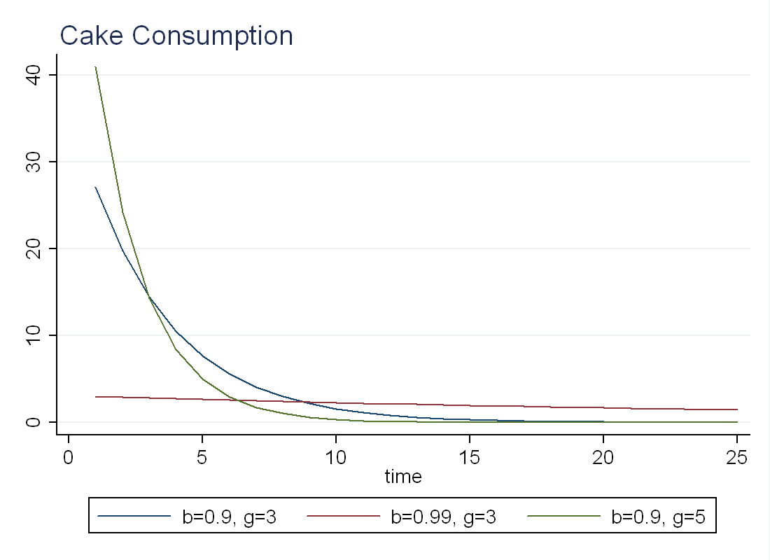
\begin{equation} c_0=(1-\beta^{\gamma}) k_0 \end{equation} \begin{equation} c_t=\beta^\gamma c_{t-1} \text{ for all }t>0 \end{equation} Below I plot the optimal consumption of a cake of size 100 for different values of \(\beta\) and \(\gamma\) (b is \(\beta\) and g is \(\gamma\)). We see that the agent with higher \(\beta\) consumes almost a constant amount of cake every day, while the agent with a high \(\gamma\) prefers to eat a large share of the cake the day he gets it.

RBC Model

First, let’s go over how to solve the RBC model (without labor) by hand. This will be the framework upon which we introduce energy consumption. The discussion here is based on class notes from Luigi Bocola’s Macroeconomics 411-3 lectures.

Equilibrium Conditions

Let uppercase letters denote quantities in levels:
Production Function: \(Y_t= e^{z_t^\alpha} K_t^{1-\alpha}\)
Law of Motion for Capital (LOK): \(K_{t+1}=(1-\delta) K_t + Y_t - C_t\)
Preferences are \(U(c_t)= \frac{c_t^{1-\frac{1}{\sigma}}}{1-\frac{1}{\sigma}}\), so the Euler Equation is: \(c_t^{-1/\sigma}=\beta E_t\Big[c_{t+1}^{-1/\sigma} R_{t+1} \Big]\)
Interest rate comes from firm FOCs (assuming firms pay for depreciation): \(R_t=(1-\alpha)e^{z_t^\alpha}K_t^{-\alpha}+(1-\delta)\)
Finally, technology is stochastic: \(z_t=\phi z_{t-1} + \sigma_z \epsilon_t\) where \(|\phi|<1\) and \(\epsilon_t\) is N(0,1).

Log-Linearize about the non-stochastic steady-state

Let lowercase letters denote log-deviations from the steady state (except for \(z_t\) which is just itself). Let uppercase letters with no subscript denote equilibrium quantities in levels.
Production Function: \(y_t=\alpha z_t + (1-\alpha) k_t\)
LOK: \(k_{t+1}=(1-\delta)k_t + \frac{Y}{K} y_t + \frac{C}{K} c_t\). Use the equation for \(R_t\) in the steady state to get \(\frac{Y}{K}=\frac{r+\delta}{1-\alpha}\) and use the expression for LOK in steady state to get \(\frac{C}{K}= \frac{Y}{K} - \delta\). Now, put this back into LOK, along with our expression for \(y_t\): \begin{equation} k_{t+1}=(1+r)k_t + \alpha \frac{r+\delta}{1-\alpha} z_t - \Big( \frac{r+\delta}{1-\alpha}-\delta \Big) c_t \end{equation} we can rewrite this as \(k_{t+1}=\lambda_1 k_t + \lambda_2 z_t + (1-\lambda-1 + \lambda_2) c_t\).
Using the fact that in the steady state, \(R=\frac{1}{\beta}\), the Euler Equation becomes: \begin{equation} \sigma E_t [r_{t+1}]=E_t[c_{t+1}-c_t] \end{equation} Log-linearizing our expression for \(R_t\), using R=1+r and our expression for Y/K from above, we get \(r_t=\frac{r+\delta}{1+r}\alpha (z_{t}-k_{t})\), putting this back into the Euler Equation we get: \begin{equation} \sigma \alpha \frac{r+\delta}{1+r}E_t[z_{t+1}-k_{t+1}]=E_t[\Delta c_{t+1}] \end{equation} where \(\Delta c_{t+1}=c_{t+1}-c_t\). We rewrite as: \(\sigma \lambda_3 E_t[z_{t+1}-k_{t+1}]=E_t[\Delta c_{t+1}]\).

Guess a Policy Function

We want to eliminate consumption from all the equations above, so we conjecture a linear policy rule: \begin{equation} c_t=\eta_{ck} k_t + \eta_{cz} z_t \end{equation} where \(\eta_{ck}\) and \(\eta_{cz}\) capture how consumption responds to current capital stock and technology, respectively.
Putting this into our LOK to eliminate \(c_t\): \begin{equation} k_{t+1}=(\lambda_1 + (1-\lambda_1 -\lambda_2) \eta_{ck}) k_t + (\lambda_2 + (1-\lambda_1 - \lambda_2) \eta_{cz}) z_t \end{equation} In addition, substitute this into our Euler Equation, and take expectations: \begin{equation} \eta_{ck} \Delta{k_{t+1}} + \eta_{cz}(\phi-1) z_t = \sigma \lambda_3 (\phi z_t - k_{t+1}) \end{equation} Where we used the fact that \(k_{t+1}\) is totally determined at time \(t\) so we don’t need expectations, and \(E_t[z_{t+1}]=\phi z_t\) from our technology process.

Solving the Model

The final work is to substitute our LOK into the Euler Equation to eliminate \(k_{t+1}\): \begin{equation} \eta_{ck}(\eta_{kk}-1)k_t+[\eta_{ck} \eta_{kz} + \eta_{cz}(\phi-1)] z_t= \sigma \lambda_3 [ \eta_{kz}-\phi]z_t - \sigma \lambda_3 \eta_{kk} k_t \end{equation} Where we used the following facts:
\(\Delta c_{t+1} = \eta_{ck} (\Delta k_{t+1}) + \eta_{cz} (z_{t+1}-z_t)\) from our conjectured policy function
\(E_t[z_{t+1}]=\phi z_t\) from our technology process
\(\Delta k_{t+1} = (\eta_{kk}-1)k_t + \eta_{kz} z_t\) from our LOK, where \(\eta_{kk}=(\lambda_1 + (1-\lambda_1 -\lambda_2) \eta_{ck})\) and \(\eta_{kz}=(\lambda_2 + (1-\lambda_1 - \lambda_2) \eta_{cz})\).
To solve the model, we set \(z_t=0\) and solve for \(\eta_{ck}\), and set \(k_t=0\) to solve for \(\eta_{cz}\). We will have two solutions for \(\eta_{ck}\) and we will choose the positive one to get a stable solution. The benefit of this formulation is that we can solve for the time series dynamics of all the variables of interest such as \(k_{t+1}\), \(y_t\) and \(c_t\).

Future Work

With the basics established, you can add the cake-eating problem to the RBC model by modifying the production function. Rather than \(Y_t=e^{z_t^\alpha}K_t^{1-\alpha}\), solve the model with \(Y_t=(e^{z_t}\zeta_t)^\alpha K_t^{1-\alpha}\) where \(\zeta_t\) is energy usage and the stock of energy follows \(S_{t+1} = S_t - \zeta_t\)