Does Adding a Constant Always Increase R-Squared?
Recall the formula for R-squared from your first statistics class:
\begin{equation}
R^2=\frac{\sum\limits_{i=1}^N (\hat{Y_i}-\overline{Y})^2}{\sum\limits_{i=1}^N (\hat{Y_i}-\overline{Y})^2 + \sum\limits_{i=1}^N (\hat{Y_i}-Y_i)^2}= \frac{SS_{model}}{SS_{model}+SS_{residual}}
\end{equation}
In that same class, you are taught that adding more regressors can not decrease R-squared, even if they have no relationship to the dependent variable.
This, however, does not apply to the constant term. At first pass, this seems hard to believe: An unconstrained model should always do at least as well as a constrained model.
The catch is, the variance explained by the constant term is not included in the calculation of R-squared - we subtract \(\overline{Y}\) when calculating \(SS_{model}\).
The no constant restriction implicitly sets \(\overline{Y}\) to zero. This will increase both the model sum of squares and the residual sum of squares. The model sum of squares effect dominates, however, and \(R^2\) is pushed towards one.
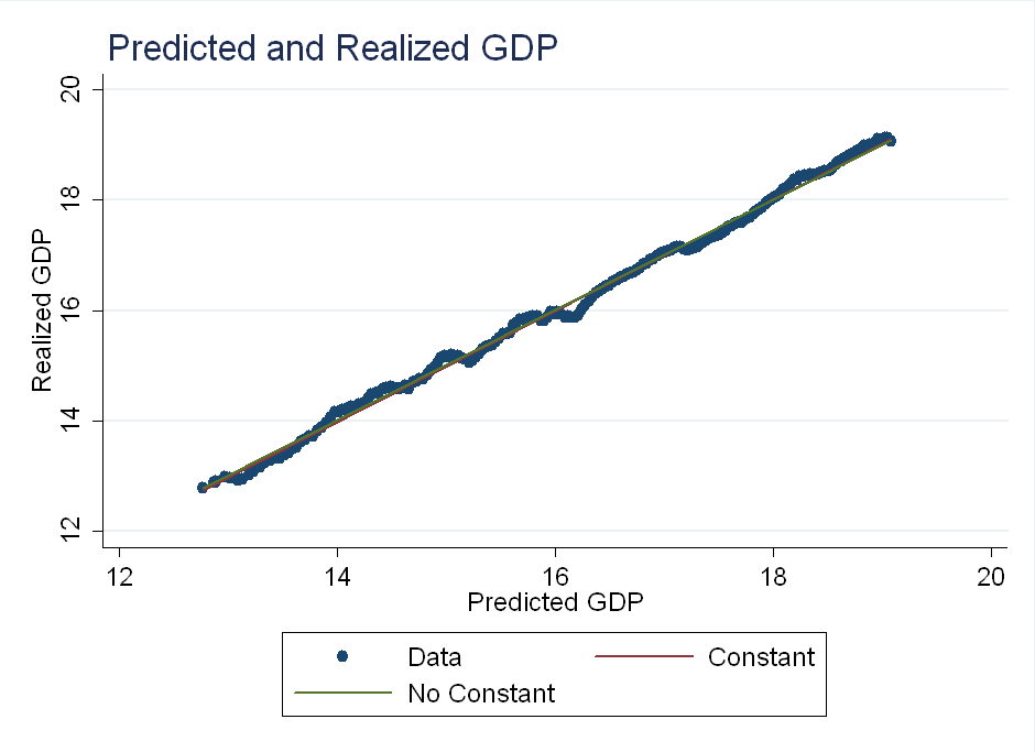
I discovered this today, regressing realized GDP on forecasted GDP. Although the sum of squared errors is nearly identical for both models, the model sum of squares is much larger for the no-intercept case:
My takeaway: Be careful when writing your own regress command in Matlab, or any other language. Omitting a constant term can drastically change R-squared.