This is the fifth post in a series on bubbles in the U.S. Equity Market. The first part can be found here.

Overview

In Part 2, we discussed the test developed by Phillips et al. to detect bubbles. As I mentioned in that post, the ADF test is basically looking for extreme return persistence. This gave me an idea - in the presence of a “bubble”, returns should become more predictable. This posts sets up a simple model and tests it empirically with the Nasdaq “bubble” discussed in Part 3.

Simple Model

Consider the classical asset pricing model, where dividends are the only fundamentals: \begin{equation} p_t = E_t \left [\sum\limits_{j=1}^\infty \beta^j \frac{u’(c_{t+j})}{u’(c_t)} d_{t+j} \right] + B_t \end{equation} Now, suppose the process for dividends follows a random walk without drift: \begin{equation} d_{t+1}=d_t + \epsilon_t \end{equation} where \(\epsilon_t\) is white noise. Further, suppose the bubble term \(B_t=0\). Under these assumptions, the stock price follows a random walk as well, so \(E_t [p_{t+1}|\Omega_t]=p_t\). In other words, our best forecast of tomorrow’s price, \(p_{t+1}\), is the price today, \(p_t\).
Now suppose \(B_t\neq0\) and \(E_t(B_{t+1})=(1+r)B_t\). With dividends still following a random walk without drift, our best forecast of tomorrow’s price is \(p_t + (1+r)B_t\). As long as the bubble persists, the bubble term should dominate the asset’s returns, and on average, the price should grow at rate \(r\) (assuming the variance of \(\epsilon\) is sufficiently small).
To convince you of this, consider a simplified model with linear utility. Then with no bubble, and using the fact that \(E_t[d_{t+j}] = d_t\): \begin{equation} p_t=E_t \Big[\beta d_{t+1} + \beta^2 d_{t+2} + \dots \Big] = \frac{\beta}{1-\beta} d_t \end{equation} Applying the law of iterated expectations: \begin{equation} E_t[p_{t+1}]=E_t \Big[\beta d_{t+2} + \beta^2 d_{t+3} + \dots \Big] = \frac{\beta}{1-\beta} d_t=p_t \end{equation} Now suppose we have a bubble: \begin{equation} p_t=E_t \Big[\beta d_{t+1} + \beta^2 d_{t+2} + \dots \Big] + B_t= \frac{\beta}{1-\beta} d_t + B_t \end{equation} Again applying the law of iterated expectations: \begin{equation} E_t[p_{t+1}]=E_t \Big[\beta d_{t+2} + \beta^2 d_{t+3} + \dots \Big] + E_t[B_{t+1}] = \frac{\beta}{1-\beta} d_t +(1+r)B_t=p_t+(1+r)B_t \end{equation} Let \(TR_i\) denote the total return of an asset over the past \(i\) periods. Then, in the presence of a bubble: \begin{equation} (TR_i+1)^{\frac{1}{6}}-1 =\hat{r} \approx r \end{equation} To test for a bubble, construct two forecasts:
1) Under no bubble: \(\hat{p}_{t+1}=p_t\)
2) With a bubble: \(\hat{p}_{t+1}=p_t(1+\hat{r})\)
Finally, (mis)use the Diebold-Mariano test to compare the forecasts (I know this is not the intended use for the Diebold-Mariano test - this will be the topic of a future blog post when I review Diebold (2013)).

Empirics

Relative Forecast Error

Before getting into the test described above, I wanted to make a first pass with some “eyeball econometrics” (a great quote from Uhlig (2005)). Note - I present all my results here, not just the ones that worked the way I wanted. Only reporting positive results and data snooping is a much bigger issue, and it will be the topic of a future blog post.

Daily Data

For now, forget the model. Suppose we only use the idea that returns become more predictable in a bubble. Using daily data run the following regression:
\(r_t = \hat{\beta} y_{t-1} + \hat{\gamma}_1 r_{t-1} + \dots + \hat{\gamma}_p r_{t-p} + \epsilon_t\)
where \(r\) is returns and \(y\) is the level (for example - the value of the Nasdaq or S&P 500 index). Use this to forecast \(\hat{r}_t\), and then forecast \(\hat{y_t}=y_{t-1}(1+\hat{r}_t)\).
The exact procedure I used is:
1) Select \(p=2\) based on AIC and BIC 2) Use a 30 day rolling window to run the regression and calculate a one-step-ahead forecast
3) Compute the relative forecast error as \(\frac{|y_t-\hat{y}_t|}{y_t}\)
4) Take a 30 day moving average of forecast error to remove noise
In the figure below, the first observation for \(y_t\) is normalized to 100.

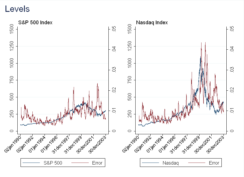
The result here is counterintuitive. Although we think returns become more predictable during a bubble, the forecasting actually gets worse! A possible explanation is that in a bubble, growth is exponential, rather than linear, so I repeated the exercise with \(y_t'=ln(y_t)\). The results are very similar.

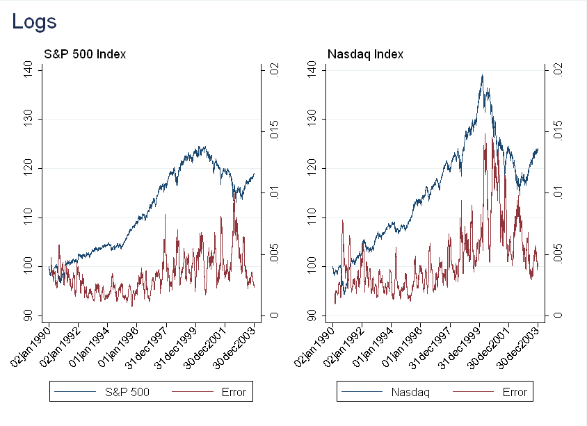
Given these two failures, I was worried that the data might be too noisy at the daily frequency to get good predictions (recall in Part 3 I discussed how the volatility of the index was very high at the time). The next section repeats the exercise with monthly data.

Monthly Data

The plot below is computed using the same methodology as above, except I did not smooth the error:

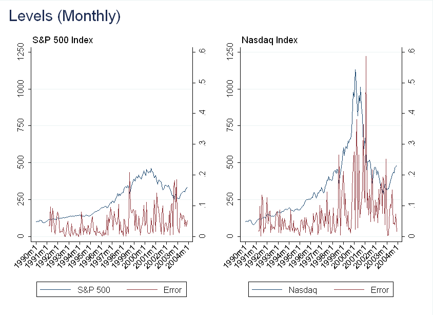
You can see there is still a large relative error during the bubble, but it is also very volatile. Smoothing the error at the quarterly frequency (using two prior months and current month) we get:

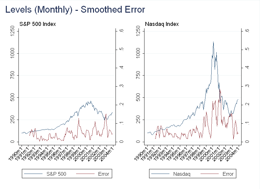
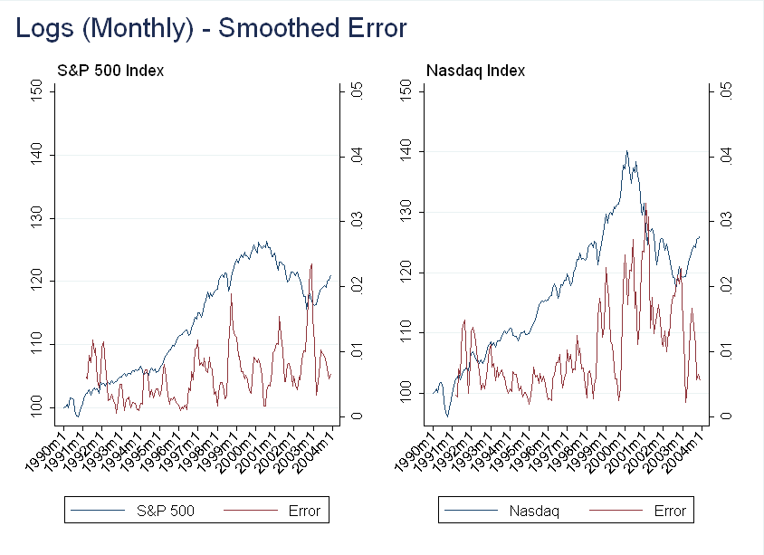
Now, this is interesting - we get a dip in the forecasting error in the middle of 1999. I don’t think it’s worth reading into this too much (as I had to do several transformations before finding this result), but there may be something here.

Forecasting Performance

Given the results above, it doesn’t seem like returns will be much more predictable during a bubble. That being said, I still think it is a worthwhile exercise to test the model described above.
The procedure I used to calculate forecasts is as follows:
1) Use 6 months of data to compute \(\hat{r}\)
2) Compute two forecasts, one being \(\hat{y}_t^1=y_{t-1}\) and \(\hat{y}_t^2=y_{t-1}(1+\hat{r})\)
3) Use the Diebold-Mariano test to compare the two forecasts
Doing this for 1998-2001 (inclusive), the random walk is better (at the 5% level) for forecasting the S&P 500 than the bubble model. For the Nasdaq, the forecasts are not significantly different at the 5% level (although the random walk model is better at the 10% level).
As above, there is not much of a difference, but there is a difference. I don’t think it makes sense to go too much further down this route without better theoretical justification, as at some point we are just data snooping.

Conclusion

Although the results were not what I expected, they are unsurprising. During a bubble we don’t just have high returns, but volatile returns as well. Even if returns become more predictable, this is obscured by high volatility.