Momentum Overview

Momentum is a simple strategy. Look at the past 12 months and identify which stocks went up the most (the winners) and which stocks went down the most (the losers). Suppose we look at all NYSE stocks between 1990 and 2015. Buying the top 10% of winners and shorting the worst 10% of losers yields an average monthly return of about 1% (this is about 13% annually) while the S&P 500 yielded an average monthly return of about 0.5% (this is about 6% annually) over the same period.
Momentum, however, has a problem - it is susceptible to crashes.
Using the guide here I was able to replicate Professor Daniel’s momentum portfolios. Using his methodology, I constructed the winner minus loser (WML) portfolio described above. Below I’ve plotted the value of 100 dollars invested in WML and 100 dollars invested in the S&P 500 on January 1st 1990. Although momentum returns higher on average, the excess returns were wiped out in 2009 during a large momentum crash.

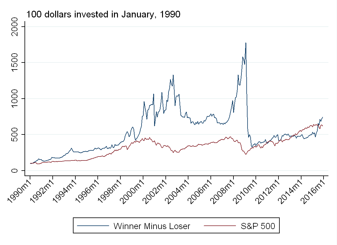
If you have been reading my posts on bubbles, you will also notice there was a momentum crash around the time the Nasdaq “bubble” collapsed (the near vertical line in 2001). This makes sense. The stocks that went up the most were probably overvalued technology stocks (even on NYSE) so when these stocks fell, momentum fell with it.
Another point to make is the relationship between bubbles and momentum. As I mentioned in Part 2 of the bubbles series, the ADF test is basically a test for return persistence. Momentum relies on return persistence to make money. A more rigorous treatment of this idea will be the topic of a future post.

Sharpe Ratio

Before getting into the paper, I wanted to review the concept of Sharpe-ratio, as the authors use it to evaluate the performance of their trading strategy. The Sharpe ratio is designed to measure the risk-adjusted return of an asset. Higher ratios indicate higher return for a given level of volatility. Higher ratios indicate a more efficient portfolio (in the mean-variance sense) - but this will be the topic of a future post.
The Sharpe ratio is of asset \(i\) is: \begin{equation} \frac{E(R_i)-r_f}{\sigma_i} \end{equation} where \(R\) denotes returns, \(\sigma\) denotes standard deviation of returns and \(r_f\) is the risk free rate. Sharpe ratio is a better way to compare assets than average returns, owing to the normalization by volatility. Intuition: an asset that returns 10% a year for sure is preferable to an asset that returns 20% half the time, and 0% half the time. Both assets have the same expected return, but the first has a higher Sharpe ratio.
Using monthly data between 2010-2015 from FRED, and setting \(r_f\)=0, I computed Sharpe ratios for 3 popular assets:
1) S&P 500: \(E(R)\)=0.009, \(\sigma\)=0.0287, Sharpe=0.312
2) BBB Total Return Index: \(E(R)\)=0.005, \(\sigma\)=0.010, Sharpe=0.442
3) AA Total Return Index: \(E(R)\)=0.004, \(\sigma\)=0.008, Sharpe=0.433
Even thought the S&P average returns are double that for BBB and AA bonds, it has a lower Sharpe ratio, owing to higher volatility.

The Paper

Summary

The authors build a model to explain the poor performance of some high past return (also called, “high momentum”) stocks. In the model, agents receive a noisy signal about the value of a risky asset, but short sale constraints prevent pessimists from selling. This drives the price above the fundamental value in the short run, but eventually, uncertainty is resolved and the asset price goes back down. Note, this has the flavor of bubbles in Barberis et. al. (2015), which will be the topic of a future blog post.
Empirically, going short the “overpriced” winners and long other winners generates Sharpe ratio of 1.08 between 1990 and 2015. This is very impressive, considering the Sharpe ratio of the S&P over the same period was less than half that.
More importantly, this excess return is not explained by common asset pricing factors, with a Fama-French 3-factor alpha of 2.71% per month.

The Model

In the model, there are two types of agents:
1) Passive investors (meant to represent institutional investors) who lend out shares in a competitive market. Their demand is not sensitive to prices.
2) Speculators, who receive a signal, \(\theta\), about the value of the risky asset. The signal is uniformly distributed around the truth, so the speculators are correct on average. Call the signal’s CDF \(F(\cdot)\) Note that by construction, half of the speculators are “optimists” and half are “pessimists.” Also, the speculators know that they have a different \(\theta\) than other speculators, but believe their signal is correct.
To short, you have to borrow. If lending supply exceeds lending demand, borrowing is costless, but if not, borrowing is costly (the authors frame this as a search cost). Call the cost of shorting \(c\).
There are three periods in the model:
Time 0: No signals received yet, no disagreement about the price so speculators stay out
Time 1: Speculators receive their signals and enter the market
Time 2: Uncertainty is resolved.
At time 1, speculators with signal \(\theta>p\) buy \(\delta\) shares, where \(\delta\) represents liquidity constraints of the speculators. Speculators who expect to make money net of shorting costs (\(c<p-\theta\)) go short. In other words, a fraction \(F_{\theta}(p-c)\) of speculators short.
To understand how many “pessimists” stay in the market, we need to understand the dynamics \(c\). The cost of shorting is decreasing in institutional lending supply and increasing in (1) divergence of opinion (bound of uniform distribution) (2) the speculators budget constraint \(\delta\) and (3) cost of searching.
The market clearing price is \(p=1+g(c)\), with \(g(0)=0\) and \(g'(c)>0\). For any \(c>0\), this is greater than the “fundamental” value of 1. The model predicts that with a restricted supply of shares \(p_1>p_0\), but \(p_2<p_1\)

Empirical Work

The authors want to figure out which stocks are expensive to short, but do not have data on actual shorting costs. Given the model above, institutional ownership and difference of opinion (defined below) should approximate shorting cost well. Using data from 1989 to 2014, the authors form 5x5x5 (125 triple-sorted) portfolios based on:
1) Past returns (momentum)
2) Institutional ownership
3) Difference of opinion, measured as simultaneous increase in short interest and price
All of these are calculated over \(t-12\) to \(t-1\) to avoid look-ahead bias.
Based on the model, the stocks that are most likely to be overpriced are those with high past returns, low institutional ownership and high difference of opinion. The authors find these stocks lose about 20% of value in the 4-5 years following portfolio formation. They use this to create a trading strategy: Based on the 5x5x5 sort, there are 25 high momentum portfolios. Go short on the high momentum portfolio with the lowest institutional ownership and the highest difference opinion, and go long the other 24 winner portfolios. To see the power of their strategy, see Figure 5 from their paper reproduced below.

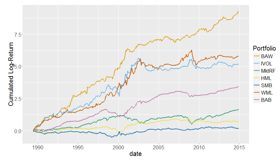
Betting against winners avoids the momentum crashes that can be seen in WML (the orange line), and outperforms many well known strategies such as Betting Against Beta (BAB - the pink line) and Value (HML - the orange line). Note - the effect of the momentum crash in WML is less dramatic in their figure because they are only forming 5 momentum portfolios, as opposed to 10, which is what I did in the Momentum overview.

Discussion

The results in the paper are pretty amazing. By doing a simple triple sort on publicly available data (does not require proprietary data on shorting costs), they are able to avoid crashes associated with momentum. That being said there are a few points I wanted to make about the paper:
1) In the model, all traders are equally (un)informed. I think it would be interesting to see if the model predicts an equilibrium price greater than the fundamental price in the presence of some fully informed traders. The authors claim that adding this wouldn’t change the model, as informed traders would only short if it was profitable net of costs (same as speculators with a low \(\theta\)). I’m not so convinced, however, as uninformed traders might “learn” from the trades of the informed guys, and put less weight on their own signal.
2) I think this raises a bigger issue with any of these types of models - why are uninformed traders in the market in the first place? In this model, all of the “optimistic” traders lose money. In fact, when you account for the distribution of signals and the cost of shorting, all traders (in expectation) lose money. In the real world, I don’t think anyone would invest in an asset if they expected to lose money. Perhaps we need a more robust model of entry and exit to account for the presence of these uninformed traders.
3) Data snooping - Any time you form 125 portfolios, you are going to get some that are sparse. Sometimes their portfolios have as few as 16 stocks. I would be curious if their result was robust to a 3x3x3 sort (only 27 portfolios), as maybe there are a few stocks driving their main result.
4) Feasibility - Their strategy talks about shorting these overpriced winners, but the whole point of the paper is that these should be hard to short!

Conclusion

Despite the issues raised above, I think the paper is still provides a compelling explanation for momentum crashes: high shorting costs prevent the market from keeping prices in line with fundamentals.