Identically Distributed (i.i.d.)

Consider a sequence of random variables: \(\{X_i\}_{i=1}^\infty\). The \(X_i\) are mutually independent if for any finite subset \(X_1,\dots,X_n\) and any finite sequence of numbers \(a_1,\dots,a_n\): \begin{equation} P \left[ \bigcup\limits_{i=1}^{n} (X_i\leq a_i) \right] = \prod\limits_{i=1}^{n} P(X_i\leq a_i) \end{equation} This may look more familiar if you replace \((X_i\leq a_i)\) with \(A_i\), an arbitrary event related to the realization of \(X_i\).
If each \(X_i\) has the same probability distribution and all \(X_i\) are mutually independent, then we say the \(X_i\) are \(i.i.d.\) An example is a sequence of coin flips - the realization of each flip does not depend on any of the previous flips, nor will it affect future flips. If a coin comes up heads 100 times in a row, the probability of heads on the next flip is still 1/2 (assuming the coin is fair, but even if it isn’t, the sequence of flips will still be \(i.i.d.\)!).

Are SPY Returns \(i.i.d.\)?

Many papers in finance treat stock returns as \(i.i.d.\) A simple example is modeling stock prices, \(p_t\), as a random walk: \begin{equation} p_t=p_{t-1} + \epsilon_t \end{equation} where \(\epsilon_t\), the returns, are \(i.i.d.\) with mean \(0\) and variance \(\sigma^2\) (not necessarily normal).
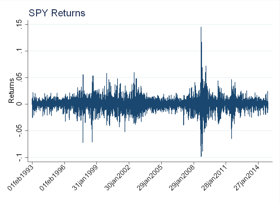
SPY is a popular ETF that tracks the S&P 500 index. Looking at daily SPY returns (the \(\epsilon_t\)’s), we see that volatility, \(\sigma^2\), is changing over time. Around the technology “bubble” in 2000 and the financial crisis in 2008, the magnitude of returns is much larger than the rest of the sample (this is called volatility clustering).

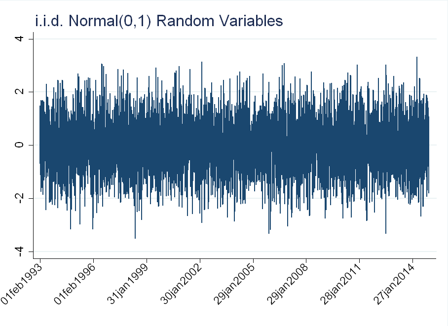
Compare this to a drawing from a Normal(0,1) distribution for each day in the sample (an \(i.i.d.\) series). There is such volatility clustering:

Time Varying Volatility

The plots above suggest volatility is time varying. To account for this, we can model \(\epsilon_t\) as a GARCH(1,1) process: \begin{equation} \epsilon_t=z_t \sigma_t \end{equation} \begin{equation} \sigma_t^2 = \omega + \alpha \sigma_{t-1}^2 + \beta \epsilon_{t-1}^2 \end{equation} where \(z_t \sim N(0,1)\).
The unconditional variance of \(\epsilon_t\) is: \begin{equation} Var(\epsilon_t)=E[\sigma_t^2 z_t^2] =E[\sigma_t^2] \end{equation} \begin{equation} = \omega + \alpha E[\sigma_{t-1}^2] + \beta E[\epsilon_{t-1}^2] \end{equation} \begin{equation} =\omega + (\alpha +\beta) E[\epsilon_{t-1}^2] \end{equation} Where the last equality follows from \(E[\epsilon_t^2]=E[\sigma_t^2]\). 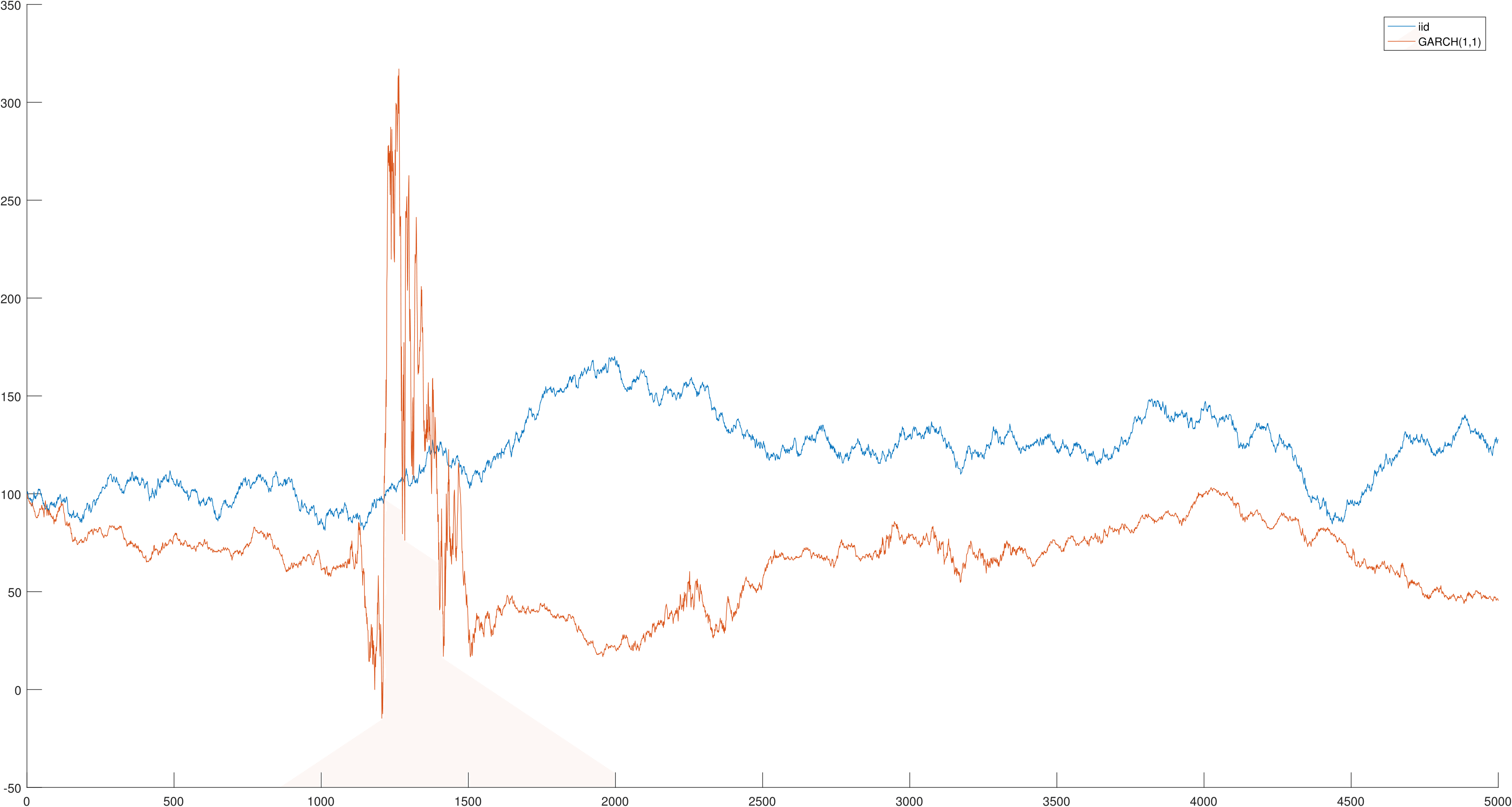We then apply the stationarity of \(\epsilon_t\) (\(\alpha+\beta<1\)) and get: \begin{equation} Var(\epsilon_t)=\frac{\omega}{1-\alpha-\beta} \end{equation} The figure below shows simulated paths for a random walk with \(iid\) standard errors (blue), and with GARCH(1,1) standard errors (orange). The GARCH parameters are calibrated to daily SPY data. In both series, the unconditional variance of \(\epsilon_t\) is the same. The GARCH series seems to exhibit a “crisis” at \(t=250\). This is not just cherry-picking, and can be replicated by seeding random numbers in MATLAB - use “rng(1,’twister’)” for the \(iid\) case and “rng(2,’twister’)” for the GARCH case.

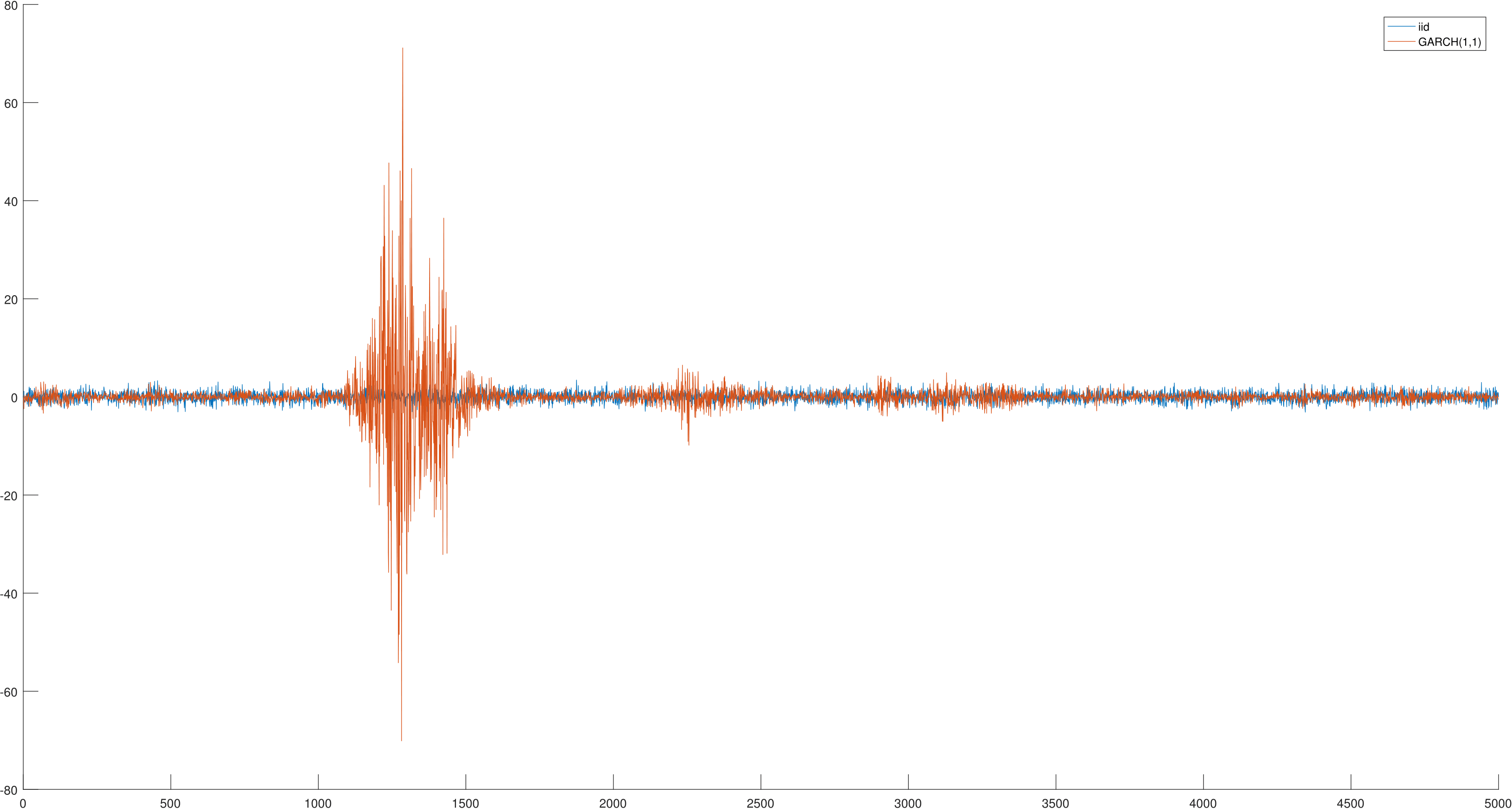
The figure below shows the innovations (the \(\epsilon_t\)’s) for both series. The GARCH(1,1) model generates volatility clustering, similar to that observed in the SPY returns, while the \(i.i.d.\) model does not.

Cleaning for Volatility

Stock returns are not \(iid\), but we can normalize them using intraday data to make this assumption roughly correct. Let \(r_{i,t}^d\) denote the daily return for stock \(i\) at time \(t\), while \(r_{i,w}\) denotes the return in a 5-minute window \(w\). We normalize returns as follows: \begin{equation} r_{i,t}^{norm}=\frac{r_{i,t}^d}{\sqrt{\sum\limits_{w \in t} r_{i,w}^2}} \end{equation} 5-minute returns are computed using TAQ trade data from 1993-2014. The following filters are applied:
1) Remove all trades with trade condition “Z” (out of sequence)
2) Only consider trades between 9:30 AM and 4:00 PM EST
3) If there are no trades in a 5-minute window \(w\), set \(r_w\)=0

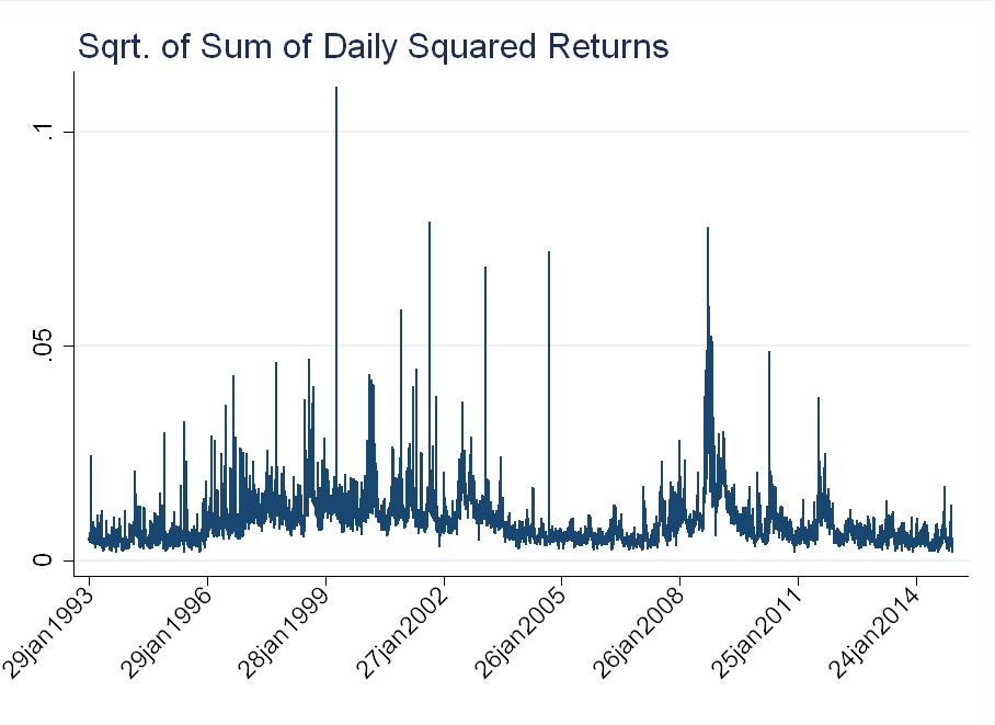
The figure below shows the evolution of \(\sqrt{\sum\limits_{w \in t} r_{i,w}^2}\):

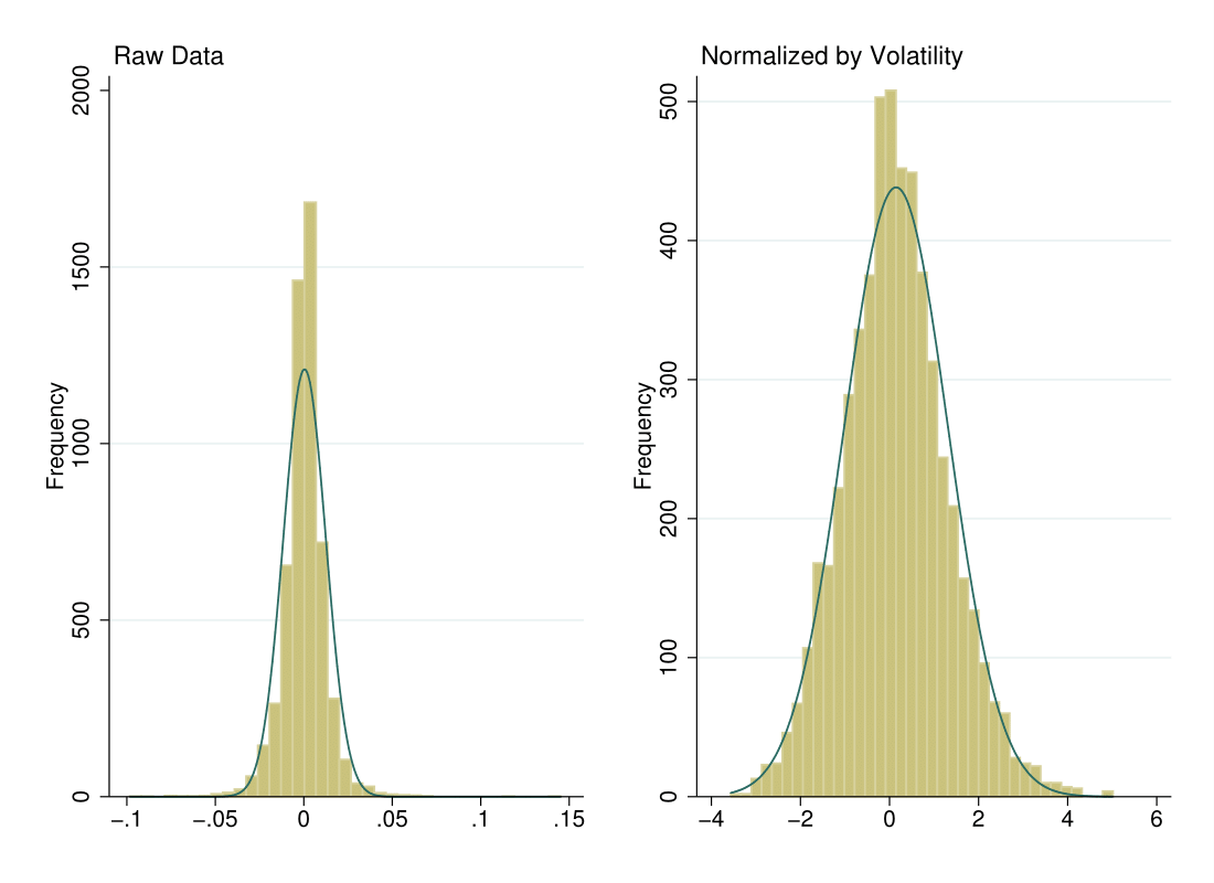
The figure below shows the distribution of returns before and after the normalization. The blue line is a normal distribution with mean and standard deviation corresponding to each series. The raw data exhibits a lot of kurtosis (the peak around 0 is very “sharp”), while much of this is alleviated in the normalized data.

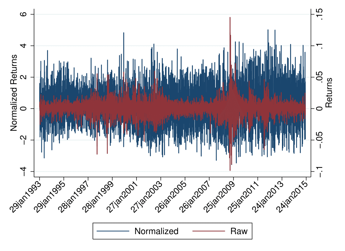
If we superimpose the volatility-cleaned return series over the realized return series, we can see that the volatility clustering has essentially been eliminated.

Price Path in an \(i.i.d.\) world

Let \(\mu_n\) and \(\sigma_n\) be the mean and standard deviation of the normalized returns, \(r_n\), while \(\mu_r\) and \(\sigma_r\) are the mean and standard deviation of daily returns, \(r\). Apply the following transformation, so the normalized returns have the same mean and standard deviation as realized returns: \begin{equation} \tilde{r}_n=\frac{\sigma_r}{\sigma_n}\left[r_n - \mu_n + \frac{\sigma_n}{\sigma_r} \mu_r \right] \end{equation}
Applying this transformation to monthly return data, we can recover the price path under the volatility-adjusted returns.

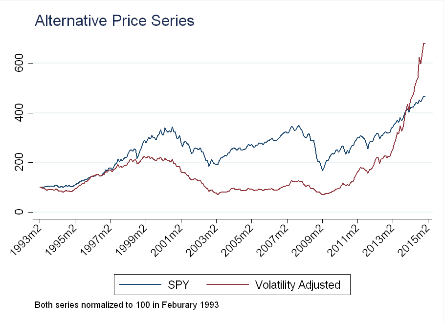
The dip after the financial crisis is dampened by high realized (intraday) volatility, while recent returns have been amplified by low realized volatility.