Are asset pricing results driven by the short side?
Return-based asset pricing factors are usually constructed as a zero cost portfolio: It is the equal weighted average of long and short positions. This discussion explores how factors are influenced by the long and short pieces in their construction. The factors are almost identical to those described on Ken French’s website.
Data Sources
The monthly stock data is from CRSP, and the quarterly fundamentals data is from Compustat. For all portfolio sorts, I use NYSE, AMEX and Nasdaq stocks with share codes between 10 and 11 (ordinary common shares for companies incorporated inside the U.S.).
6 Portfolios Formed on Size and Book-to-Market
To be included in one of these portfolios, a stock must meet the following conditions at t-1 (the end of the previous month): Non-missing return, non-missing shares outstanding, non-missing/stale price and non-missing/negative book value of equity (computed as Common Equity + Deferred Tax and Investment Tax Credit - Preferred Stock).
To avoid a look-ahead bias, a 6-month lag is imposed between the end of the fiscal quarter and the use of the book value data. For example: if a company’s fiscal year ends in December, the Q2 data is used to form portfolios at the end of Q4. Book value of equity is updated annually.
Every month, I calculate the median market capitalization, as well as the 30th and 70th percentile of B/M ratio (book value of equity/market value of equity) using only NYSE stocks. I then apply these breakpoints to all NYSE, AMEX and Nasdaq stocks of interest.
Stocks with below median market capitalization are small, while the rest are big. Stocks in the bottom 30% of B/M are growth stocks, while the top 30% are value stocks, the rest are neutral.
Portfolios are rebalanced monthly and are value weighted (using the end of the previous month’s market capitalization).
6 Portfolios formed on size and momentum
To be included in one of these portfolios, a stock must meet the following conditions at t-1 (the end of the previous month): Non-missing shares outstanding, non-missing/stale price, non-missing t-2 return & non-missing/stale t-13 price (t-1/t-12 from the standpoint of the formation period i.e. the end of the previous month), and at least 13 months of historical data.
Every month, I calculate the median market capitalization, as well as the 30th and 70th percentile of the t-12 to t-2 cumulative returns (i.e. \((1+r_{t-2})(1+r_{t-3})\dots(1+r_{t-12})\)) using only NYSE stocks. I then apply these breakpoints to all NYSE, AMEX and Nasdaq stocks of interest.
Stocks with below median market capitalization are small, wile the rest are big. Stocks in the bottom 30% of past returns are low momentum stocks, while the top 30% are high momentum stocks, the rest are neutral.
Small Minus Big (SMB)
This factor is designed to capture the size effect - that small stocks have historically performed better than large stocks. I compute SMB in line with Ken French’s methodology, using the 6 portfolios formed on size and book-to-market:
SMB = 1/3 (Small Value + Small Neutral + Small Growth) - 1/3 (Big Value + Big Neutral + Big Growth).
High Minus Low (HML)
This factor is designed to capture the value effect - that high B/M stocks have historically performed better than low B/M stocks. I compute HML in line with Ken French’s methodology, using 4 of the 6 portfolios formed on size and book-to-market:
HML = 1/2 (Small Value + Big Value)- 1/2 (Small Growth + Big Growth).
Momentum (MOM)
This factor is designed to capture the momentum effect - stocks that went up the most over the previous 12 months have historically performed better than the stocks that went up the least. I compute MOM in line with Ken French’s methodology, using 4 of the 6 portfolios formed on size and momentum: MOM = 1/2 (Small High + Big High)-1/2(Small Low + Big Low).
The Market
The market return is computed as the value-weighted return of all ordinary common stocks traded on the NYSE, AMEX, or Nasdaq. To be included in the market portfolio, a stock must meet the following conditions at t-1 (the end of the previous month): Non-missing return, non-missing shares outstanding, non-missing/stale price.
The Factors
Below I plot the small and big portfolios as well as the SMB factor:
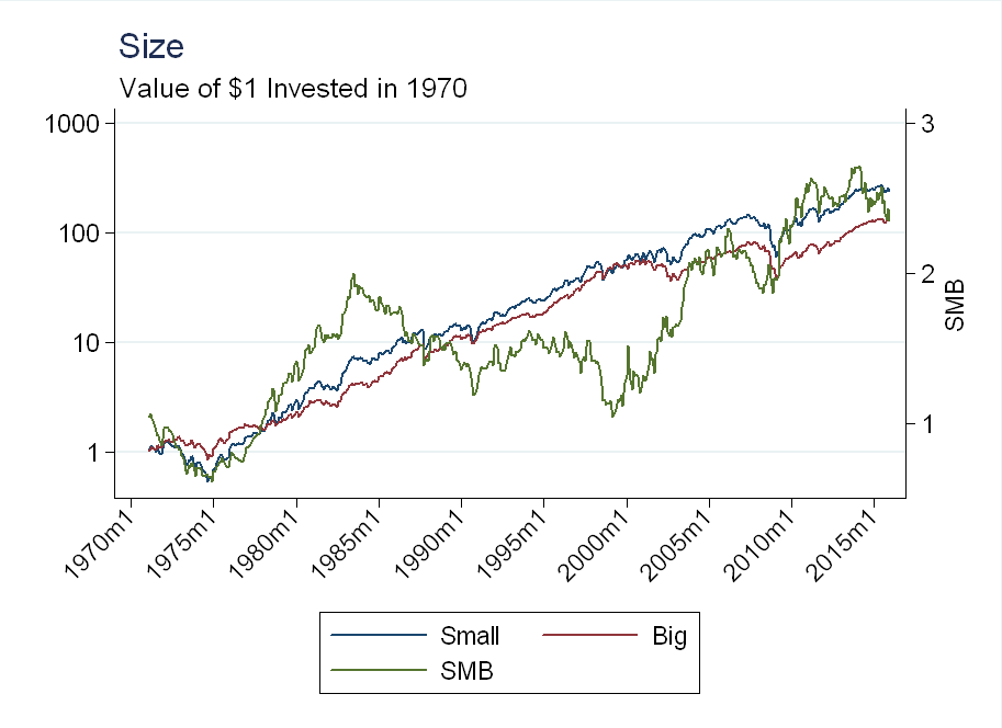
Small stocks performed better than big stocks from about 1975-1985, but the effect reversed from 1985-2000. From 2000-2008 the size effect returned, but it weakened, and reversed again after the financial crisis.
Similar to above, I plot the value and growth portfolios as well as the HML factor:
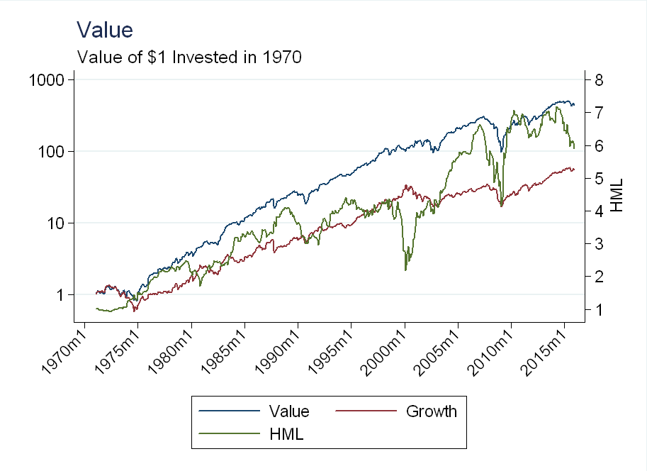
Note the difference in scale on both the left and right axis. The value effect is “stronger” than the size effect, in that the value stocks have gone up a lot more than small stocks. There have been a few value “crashes” associated with the technology bubble and the financial crisis. These are not surprising: in the technology bubble growth stocks went up a lot (only to come back down soon after), while value stocks hardly moved. As for the financial crisis: A stock might have a high B/M ratio owing to a weak balance sheet. When the crisis hit, many of these weak firms might have exited, or continue to perform poorly.
Finally, I plot the high and low portfolios as well as the MOM factor:
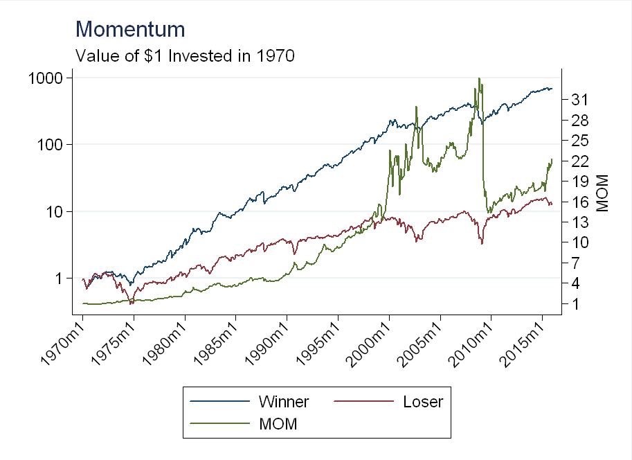
As you can see, there are two major momentum crashes, whose timing lines up the the value crashes (the relationship between the two is discussed in Value and Momentum Everywhere, by Asness et. al. 2013). Again, these are not surprising, as technology stocks in the 2000’s were high momentum, and they all crashed around the same time.
The Long/Short Side
Below, I compare the performance of the small and big portfolios to the market as a whole:
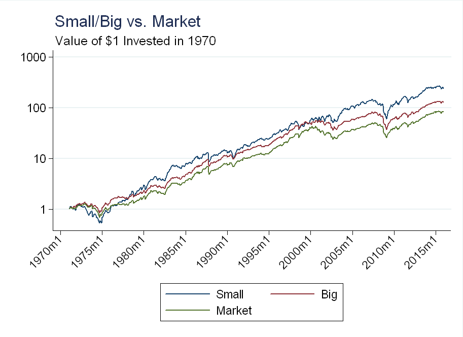
Initially, I thought it was strange that both could outperform the market, but it has to do with the weighting. The small and big portfolios are an equal weighted average of 3 value weighted portfolios. This is different than a value-weighted average all the stocks in the 3 portfolios combined. As a result, small stocks are getting “too much” weight in the big portfolio (a way to “fix” this would be to just take a value weighted average of the top 50% of stocks by market capitalization).
As for the long vs. short side, there is not much here, both portfolios outperform the market, but small does slightly better than big.
We see a larger difference with the value and growth portfolios:
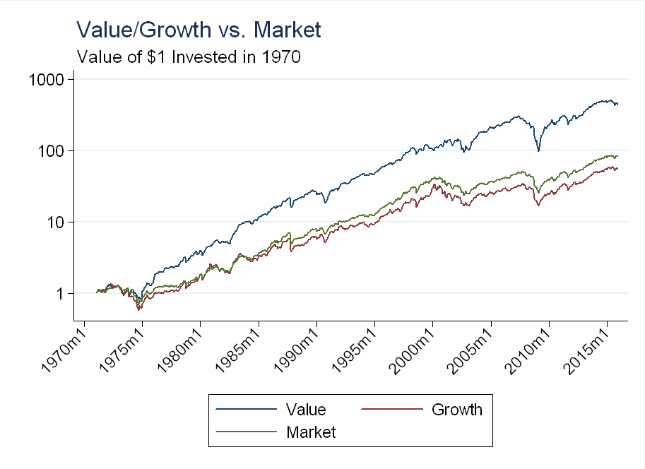
The growth portfolio underperformed the market, although not by that much. The value factor is mostly driven by the long side - The market was up about 100x over this time period, while value was up about 500x.
Finally, we see the most dramatic difference for the momentum portfolios:
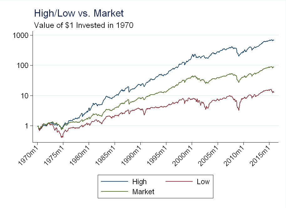
The market went up almost 100x, while the low significantly underperformed at about 10x. The long side was up about 700x, so I conclude both the long and short effects are significant here.
Conclusion
While the short side doesn’t contribute much to the size factor, it has some influence on the value factor and a large influence on the momentum factor. Given that shorting can be expensive or impossible (especially on some of the loser stocks which are small and/or illiquid) it’s unlikely a trader could actually realize the momentum factor returns. This is one reason why momentum is better viewed as a ‘sytle’ factor, rather than a ‘fundamental’ factor.