This post is based on problems 2.10 and 2.11 in, “Heard on the Street” by Timothy Falcon Crack. I was asked how to price a digital option in a job interview - and had no idea what to do!

European Call Options

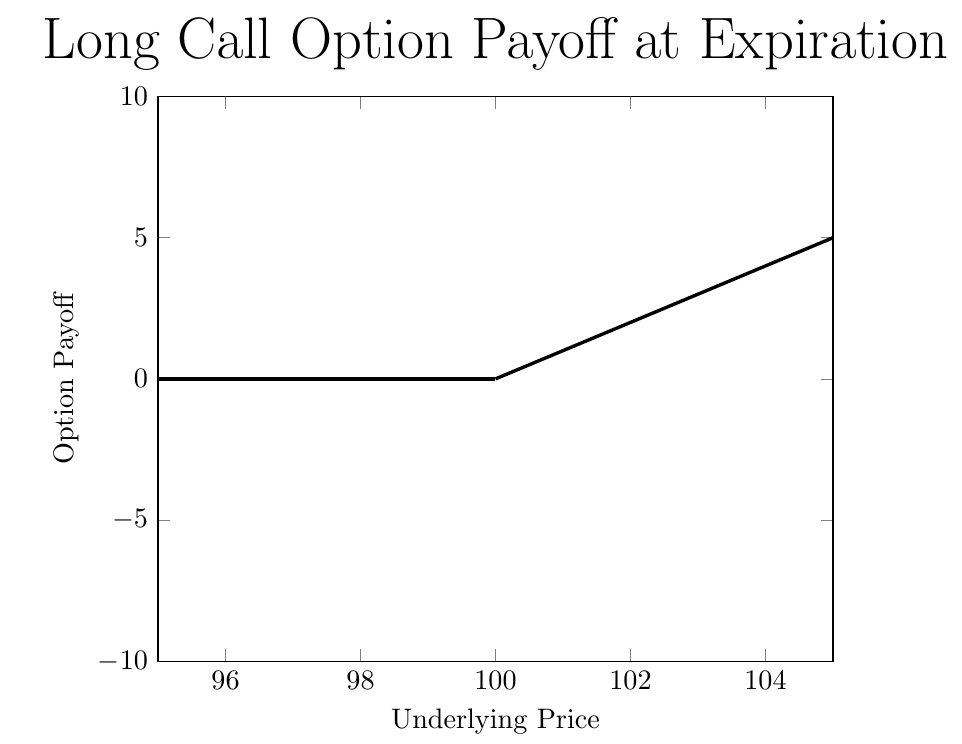
A European call option is the right to buy an asset at the strike price, \(K\), on the option’s expiration date, \(T\). A call is only worth exercising (using) if the underlying price, \(S\), is greater than \(K\) at \(T\), as the payoff from exercising is \(S-K\). The plot below shows the value of a call option, as a function of the underlying asset’s price, with \(K=100\):

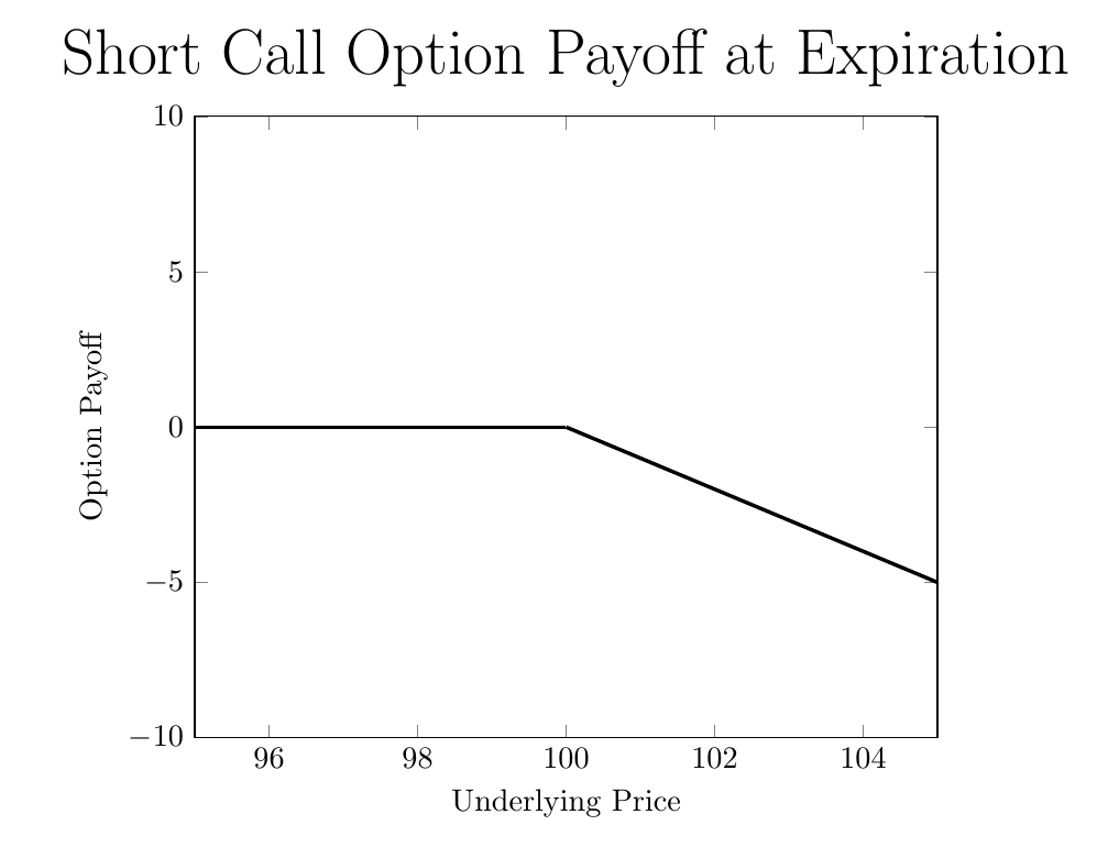
Selling a call option with a strike \(K=100\) earns you the call’s price, \(c\), today, but your payoff will be decreasing in the underlying price:

Digital Call Options

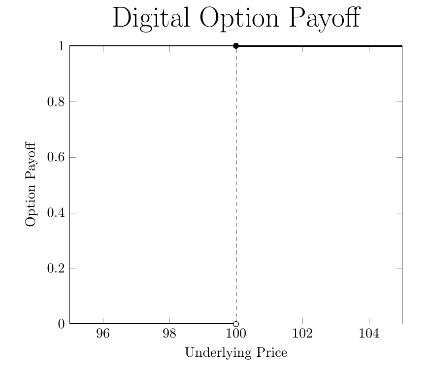
A digital call option with \(K=100\) is similar - it pays off one dollar if \(S\geq100\) at expiration, and pays off zero otherwise:

Suppose you have a model for pricing regular call options. If you’re using Black-Scholes the price of the call, \(c\), is a function of \(K\), \(S\), time to expiration \(T-t\), the volatility of the underlying asset \(\sigma\), and the risk free rate \(r\): \begin{equation} c=F(K,S,T-t,\sigma,r) \end{equation} Now - suppose the model is correct. How can you use \(F(K,\cdot)\) to price the digital option?

Replicating the Digital Option

The trick is to replicate the digital option’s payoff with regular calls. As a starting point, consider buying a call with \(K=100\) and selling a call with \(K=101\):

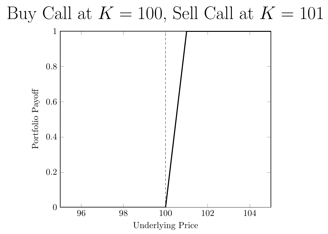
This is close to the digital option, but not exactly right. We want to make the slope at 100 steeper, so we need to buy more options. This is because a call’s payoff increases one-for-one with the underlying once the option is in the money, so with one option you are stuck with a slope of one.
Consider buying two calls with \(K=100\) and selling two calls at \(K=100.5\):

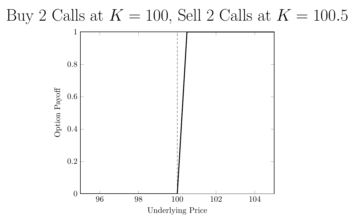
As opposed to a slope of 1 between 100 and 101, now we have a slope of two between 100 and 100.5.

Generalizing this idea - consider a number \(\epsilon>0\). To get a slope of \(\frac{1}{\epsilon}\), you buy \(\frac{1}{\epsilon}\) calls at \(K=100\) and you sell \(\frac{1}{\epsilon}\) calls at \(K=100+\epsilon\). Here’s what it looks like for \(\epsilon=\frac{1}{10}\):

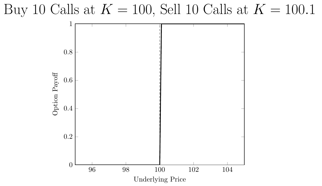
Given that the slope is \(\frac{1}{\epsilon}\), to get an infinite slope, we take the limit as \(\epsilon\) goes to zero.

How much will the above portfolio cost? You earn \(\frac{1}{\epsilon}F(100+\epsilon, \cdot)\) from selling the \(K=100+\epsilon\) calls, and pay \(\frac{1}{\epsilon}F(100, \cdot)\) for the \(K=100\) calls. The net cost is: \begin{equation} lim_{\epsilon \rightarrow 0} \frac{F(100+\epsilon,\cdot)-F(100,\cdot)}{\epsilon} \end{equation}

What does this look like? A derivative! It might look more familiar if I re-wrote it as:

\begin{equation} lim_{\epsilon \rightarrow 0} \frac{F(K+\epsilon)-F(K)}{\epsilon} \end{equation}

The price of the digital option is the derivative of \(F\) with respect to the strike price \(K\).

Conclusion

Many complicated payoffs can be re-created as combinations of vanilla puts and calls. For an overview, see the first few chapters of Sheldon Natenberg’s, “Option Volatility & Pricing”.