Sims and Uhlig argue: although classical (frequentist) \(p\)-values are asymptotically equivalent to Bayesian posteriors, they should not be interpreted as probabilities. This is because the equivalence breaks down in non-stationary models.
The paper uses small sample sizes, with \(T=100\) - This post examines how the results change with \(T=10,000\), when the asymptotic behavior kicks in.

The Setup

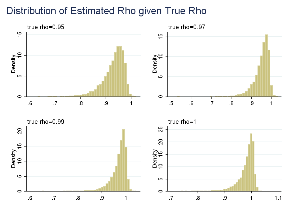
Consider a simpler AR(1) model: \begin{equation} y_t=\rho y_{t-1} + \epsilon_t \end{equation} To simplify things, suppose \(\epsilon_t \sim N(0,1)\). Classical inference suggests that for \(|\rho|<1\), the estimator is asymptotically normal and converges at rate \(\sqrt{T}\): \begin{equation} \sqrt{T}(\hat{\rho}-\rho) \rightarrow^{L} N(0,(1-\rho^2)) \end{equation} For \(\rho=1\), however, we get a totally different distribution, which converges at rate \(T\), instead of rate \(\sqrt{T}\): \begin{equation} T(\hat{\rho}-\rho)=T(\hat{\rho}-1)= \rightarrow^{L} \frac{(1/2)([W(1)]^2-1)}{\int_0^1 [W(r)]^2 dr} \end{equation} where \(W(1)\) is a Brownian motion. Although it looks complicated, it is easier to visualize when you see \(W(1)^2\) is actually a \(\chi^2(1)\) variable. This is left skewed, as the probability that a \(\chi^2(1)\) is less than one is 0.68 and large realizations of \([W(1)]^2\) in the numerator get down-weighted by a large denominator (it is the same Brownian motion in the numerator and denominator). In the paper, the authors choose 31 values of \(\rho\) between 0.8 to 1.1 in increments of 0.01. For each \(\rho\) they simulate 10,000 samples of the AR(1) model described above with \(T=100\). Finally, they run an OLS regression of \(y_t\) on \(y_{t-1}\) to get the distributions for \(\hat{\rho}\) (the OLS estimator of \(\rho\)). Below I show the distribution of \(\hat{\rho}\) for selected values of \(\rho\):

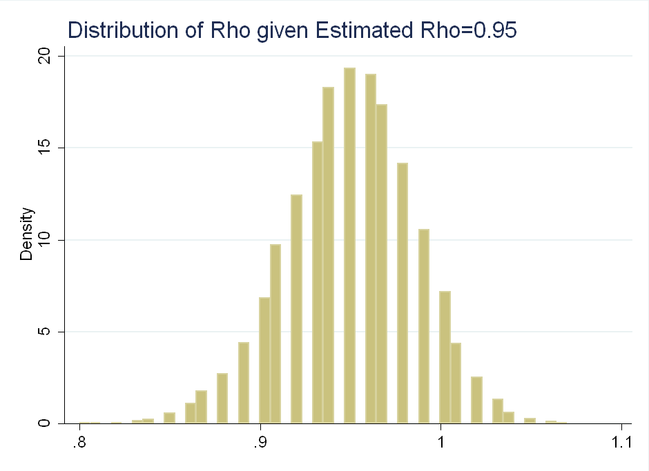
Another way to think about the data is to look at the distribution of \(\rho\) given observed values of \(\hat{\rho}\). This is symmetric about 0.95:

Their problem with using \(p\)-values as probabilities is that if we observe \(\hat{\rho}=0.95\), we can reject the null of \(\rho=0.9\), but we fail to reject the null of \(\rho=1\) (think about the area in the tails after normalizing the distribution to integrate to 1), even though \(\rho\) given \(\hat{\rho}\) is roughly symmetric about 0.95:

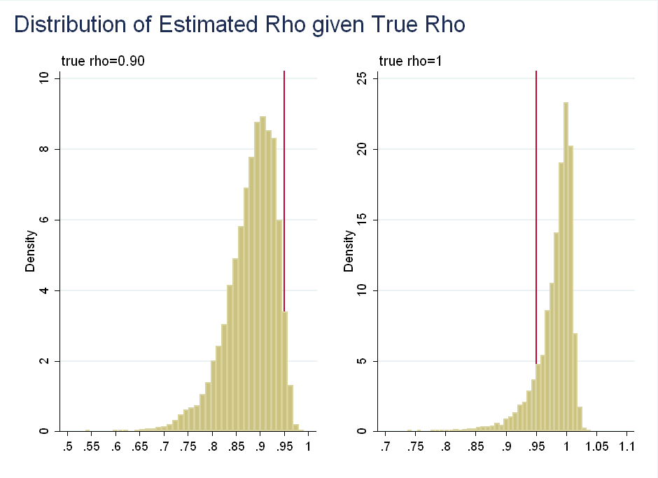
The problem is distortion by irrelevant information: Values of \(\hat{\rho}\) much below 0.95 are more likely given \(\rho=1\) than are values of \(\hat{\rho}\) much above 0.95 given \(\rho=0.9\). This is irrelevant as we have already observed \(\hat{\rho}=0.95\), so we know it is not far above or below.

The prior required to generate these results (i.e. the prior that would let us interpret \(p\)-values as posterior probabilities) is sample dependent. Usually, classical inference is asymptotically equivalent to Bayesian inference using a flat prior, but it is not the case here. The authors show that classical analysis is implicitly putting progressively more weight on values of \(\rho\) above one as \(\hat{\rho}\) gets closer to 1.

Testing with Larger Samples

At first, I found the results counter-intuitive. The first figure above shows that the skewness arrives gradually in finite samples. This is strange, because the asymptotic properties of \(\hat{\rho}\) are only non-normal for \(\rho=1\). I figured this was the result of using small samples of \(T=100\). Under a flat prior, the distribution of \(\rho\) given the data and \(\epsilon_t\) having variance of 1 is: \begin{equation} \rho \sim N(\hat{\rho}, (\sum\limits_{t=1}^T y_{t-1})^{-1}) \end{equation} This motivates my intuition for why the skewness arrives slowly: even for small samples, as \(\rho\) gets close to 1, \(\sum\limits_{t=1}^T y_{t-1}\) can be very large.

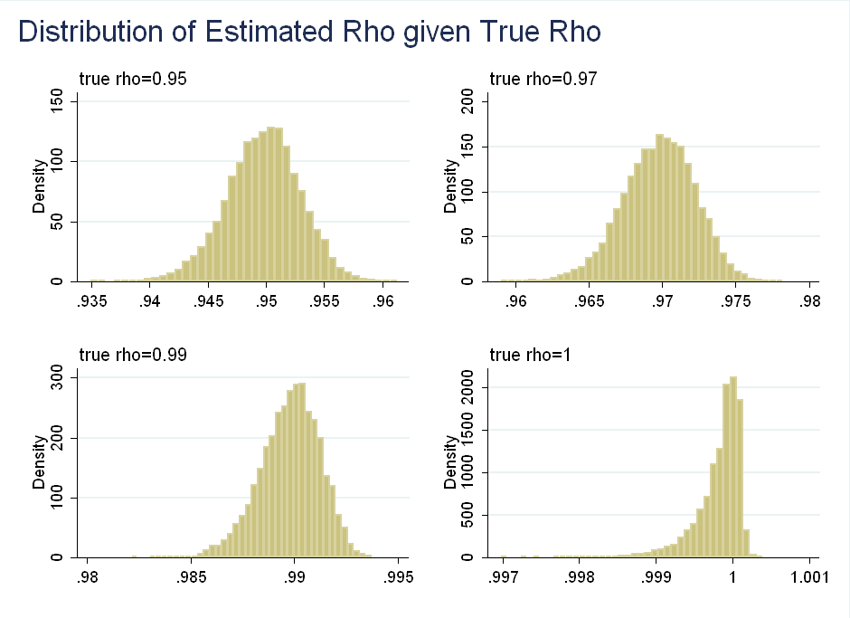
I repeat their analysis, except instead of \(T=100\), I use \(T=10,000\). As you can see, the asymptotic behavior kicks in and the skewness arrives only at \(\rho=1\):

I also found that for \(T=10,000\) the distribution of \(\rho\) conditional on \(\hat{\rho}\), does not spread out more for smaller values of \(\hat{\rho}\), that is a small sample result.

Conclusion

The point of this paper is to show that the classical way of dealing with unit roots implicitly makes undesirable assumptions - you need a sample-dependent prior which puts more weight on high values of \(\rho\). To a degree, the authors’ results are driven by the short length of the simulated series. The example where you reject \(\rho=0.9\) but fail to reject \(\rho=1\) wouldn’t happen in large samples, as the asymptotic kick in and faster rate of convergence for \(\rho=1\) gives the distribution less spread.

For now, however, the authors’ criticism is still valid. With quarterly data from 1950-Present you get about 260 observations. Macroeconomics will have to survive until year 4,450 for there to be 10,000 observations, and that’s a long way off.