Constructing a Stock Screener
Value and Momentum
Two of the most discussed effects in the asset pricing literature are Value and Momentum.
Let’s start with the definitions:
1) Value Effect: Stocks with high book-to-market have historically outperformed stocks with low book-to-market
Book-to-Market: (book value of common equity + deferred taxes and investment credit - book value of preferred stock)/(market value of equity). The higher the book-to-market (BM), the “cheaper” the stock, as you are getting more book value for every dollar you invest.
2) Momentum Effect: Stocks with high returns over the previous year (winners) have historically outperformed stocks with low returns over the previous year (losers). Past-year returns are calculated as the cumulative returns from \(t-12\) to \(t-2\) (month \(t-1\) is excluded).
Bonus – Size Effect: Stocks with low market capitalization (price \(\times\) shares outstanding) have historically outperformed stocks with high market capitalization. Both the value and momentum effects are stronger among small stocks.
Trading on Value and Momentum
Although there are many ways to construct portfolios based on the value and momentum effects, I will start with the following baseline for back-testing (see here for details):
1) Start with monthly CRSP data, and adjust for delisting returns. I do this by (1) Setting the return to the delisting return in the month that the firm delists if the delisting return is non-missing (2) Set the delisting return to -0.3 (-30%) if the delisting return is missing and the delisting code is 500, 520, 551-573, 574, 580 or 584 (3) Set the delisting return to -1 (-100%) if the delisting return is missing, and the delisting code does not belong to the list above. This is important for calculating returns in the extreme value and momentum portfolios, as these firms have a higher-than-average likelihood of delisting.
2) Each month, select ordinary common shares which have non-stale prices, non-missing returns, non-missing shares outstanding and are traded on the major exchanges (NYSE, AMEX and NASDAQ).
2a) For the value portfolios, select firms with a non-missing book-to-market.
2b) For the momentum portfolios, select firms with a non-missing/non-stale price at t-12, and no more than 4 missing returns between t-12 and t-2.
3) Select only NYSE firms, then calculate percentiles of the sorting variables among these firms each month – these are the breakpoints we are going to use to form portfolios. For example: If you want to form 5 value portfolios, calculate the 20th, 40th, 60th and 80th percentiles of book-to-market for every month in your sample.
4) Merge these breakpoints back into the rest of the data (all NYSE, AMEX and NASDAQ firms). Then sort into portfolios based on the breakpoints. Back to the five value portfolios example: Firms with a book-to-market below the 20th percentile will be put into portfolio one, firms with a book-to-market between the 20th and 40th percentiles will be put into portfolio 2, etc. Note: The portfolios will not all have the same number of firms. This is because the average NSADAQ/AMEX firm is different than the average NYSE firm, so the percentiles will not line up exactly. This prevents small firms from exerting an undue influence on the results.
5) Now you have the portfolio assignments at the end of each month. Portfolios are rebalanced monthly, so these assignments will be used for the following month to prevent a look-ahead bias.
6) All portfolios are value-weighted using last month’s ending market capitalization. This also prevents a look-ahead bias.
7) Convert each portfolio return to an excess return by subtracting the monthly risk-free rate, which can be found at Ken French’s data library.
8) Form a factor portfolio by subtracting the extreme portfolios from one another. Using the 5 value portfolio example: Subtract the 1 portfolio (lowest BM) from the 5 portfolio (highest BM). This is also an excess return. Call these portfolios high-minus-low (HML).
9) Following the observation of Value and Momentum Everywhere, form a “Combo” portfolio which is an equal-weighted average of the value and momentum portfolios. Because the value and momentum effects deliver positive excess returns, and are negatively correlated, a combination of the two should on average outperform either strategy on its own.
Evaluating Portfolio Performance
I am going to start by evaluating performance in the simplest way possible: CAPM alpha – which is a measure of average returns that cannot be explained by a portfolio’s covariance with the market portfolio.
To calculate this, run the following regression:
\begin{equation} R^e_{p,t}=\alpha + \beta R^e_{m,t} + \epsilon_{p,t} \end{equation}
where \(R^e_{p,t}\) is the excess return on the portfolio of interest, \(R^e_{m,t}\) is the excess return on the market and \(\alpha\) denotes the CAPM alpha we are trying to measure.
The table below presents the CAPM alphas and corresponding t-Statistics for 10 portfolios formed on value and momentum using data from 1970-2016. All quantities are annualized.
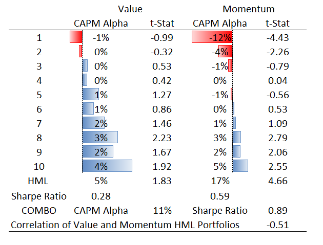
For both value and momentum, the CAPM alpha is almost monotonically increasing from the low-BM/loser portfolios to the high-BM/winner portfolios. The high-minus-low portfolios both generate positive CAPM alphas, although the CAPM alpha for value is only marginally significant. As expected, the negative correlation between value and momentum gives the COMBO portfolio a higher Sharpe Ratio (average excess return/standard deviation of excess returns) than either portfolio on its own.
Conditioning on Size
In this section I am going to use an alternative portfolio construction: At step 3 above, first divide NYSE firms into two groups – above and below median market capitalization. Then, calculate the breakpoints for value and momentum within each of these two groups. This is useful for understand how the value and momentum effects differ among large and small firms.
I then run the same CAPM regression as above. The table below presents the CAPM alphas and corresponding t-Statistics for \(2 \times 5\) portfolios formed on size and value/momentum, using data from 1970-2016. All quantities are annualized.
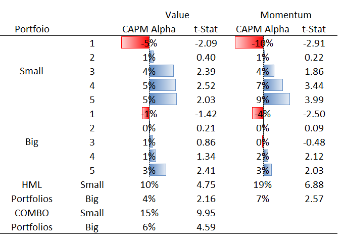
As above, the CAPM alpha is almost monotonically increasing from the low-BM/loser portfolios to the high-BM/winner portfolios within both the small and large firm groups. As mentioned previously, the CAPM alphas for value and momentum are larger for the group of smaller firms.
Next Steps
With the basics established, you can refine the stock screener by:
1) Using less stale book-to-market data
2) Accounting for mis-measurement of book-to-market with intangible assets
3) Account for heterogeneity across industries
4) Accounting for “junky” stocks that get picked up by a value filter
5) Impose restrictions, such as value-weighted portfolio beta