Bubbles: Part 2. Article Review - Testing for Multiple Bubbles by Phillips, Shi and Yu (2013)
This is the second post in a series on bubbles in the U.S. Equity Market. The first part can be found here.
Testing for Multiple Bubbles 1: Historical Episodes of Exuberance and Collapse in the S&P 500, Phillips, Shi and Yu, 2013
Summary
As mentioned previously, most bubbles are identified ex-post. This presents a problem for policy makers who would like to identify bubbles early and prevent them from growing too large. Whether or not policy makers should do this is an entirely different question and will be addressed in a future post. The focus here is to discuss a paper by Phillips et al. which implements a purely statistical technique for identifying the emergence and collapse of bubbles.
The paper is designed to fix a specific problem - other statistical techniques (including Philips 2011) fail when a series exhibits multiple bubbles of different time lengths and magnitudes. This is important, as we suspect the S&P 500 has experienced several bubble periods in the past 100 years. To this end, the authors implement the generalized sup augmented Dickey-Fuller test (GSADF), which will be discussed in more detail below.
Unit roots
Consider the ARMA(p,q) representation of a stochastic process: \(\{y_t\}_{t=0}^\infty\)
\begin{equation}
\Phi(L) y_t = \Theta(L) \epsilon_t
\end{equation}
we say the process has a unit root, when the lag polynomial \(\Phi(L)\) has a root equal to 1. In other words, a solution to \(\Phi(z)=1-\phi_1 z - \dots -\phi_p z^p=0\) is \(z=1\).
Understanding unit roots is important, because it can totally change the behavior of a stochastic process. Consider a simple AR(1) model.
\begin{equation}
y_t = \rho y_{t-1} + \epsilon_t
\end{equation}
with \(\epsilon_t \sim N(0,1)\).
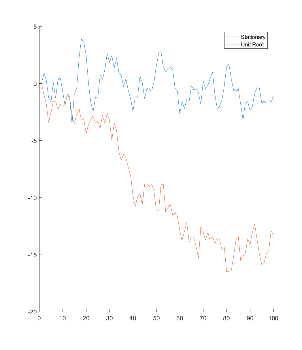
Below I’ve simulated two AR(1) series, one that is stationary (\(\rho=0.8\)), and one with a unit root (\(\rho=1\)). As you can see, the stationary series tends to revert to it’s mean, while the unit root has no such tendency.
Augmented Dickey-Fuller (ADF) Test
Before getting into the paper, I think it is important to review the ADF test for a unit root. This will help us understand what exactly Philips et al. are doing with the GSADF test. The discussion of the ADF test follows closely the treatment in Hamilton (1994).
Suppose we have an AR(p) process:
\begin{equation}
(1-\phi_1 L - \phi_2 L^2 - \dots - \phi_p L^p) y_t = \epsilon_t
\end{equation}
Now, doing some algebra, we can rearrange this as follows (with \(\Delta\) denoting the first difference operator):
\begin{equation}
y_t = \rho y_{t-1} + \psi_1 \Delta y_{t-1} + \dots + \psi_{p-1} \Delta y_{t-p+1} + \epsilon_t
\end{equation}
Now suppose our null hypothesis is that \(y_t\) is a unit root without drift (\(\alpha=0\) and \(\rho=1\)). This implies one of the roots of \((1-\phi_1 z - \dots - \phi_p z^p)\) is 1, and all the others are outside the unit circle. To implement the Dickey-Fuller test for a unit root, we estimate the following regression: \(y_t=\alpha + \hat{\rho} y_{t-1} + \hat{\psi}_1 \Delta y_{t-1} + \dots + \hat{\psi}_{p-1} \Delta y_{t-p+1} + \epsilon_t\)
Under the null \(\hat{\rho}\) will converge at rate \(T\) to a non-standard distribution, which is why the appropriate critical values are calculated by simulation. If \(\rho\) is sufficiently small, we reject the null of a unit root in favor of the left-tailed alternative (\(\rho<1\)).
The Paper
Consider adding a bubble component to our standard asset pricing equation:
\begin{equation}
P_t=E_t \left[ \sum\limits_{j=1}^{\infty} \Bigg(\frac{1}{1+r_f}\Bigg)^j (D_{t+j} + U_{t+j}) \right]+ B_t
\end{equation}
Where \(r_f\) is the risk-free rate, \(D_{t+j}\) is the dividend paid and \(U_{t+j}\) is an unobserved fundamental component at time \(t+j\). \(B_t\) is the bubble component, which follows a submartinagle: \(E(B_{t+1})=(1+r)B_t\). When \(B_t=0\), the asset price is controlled by dividends and fundamentals. Suppose \(D_t\) is integrated of order 1, meaning \(D_t\) has a unit root. Denote this I(1). Suppose further that \(U_t\) is integrated of order 0, I(0), or I(1). If this is true, then the asset price is at most I(1).
If \(B_t\neq0\) the price is explosive. This implies that explosive asset price behavior can be used to detect bubbles.
SADF
Suppose we split the sample into different windows. For example, consider running an ADF test, using only data between period \(r_1\) and \(r_2\) (so the sample size is \(r_2-r_1\)):
\begin{equation}
\Delta y_t = \alpha_{r1,r2} + \beta_{r1,r2} y_{t-1} + \sum\limits_{i=1}^k \psi_{r1,r2}^i \Delta y_{t-i} + \epsilon_t
\end{equation}
note this is equivalent to the formulation above under the null. When \(\rho=1\), we can subtract \(y_{t-1}\) from both sides to get this equation. Now, rather than testing \(\rho=1\) we are testing \(\beta=0\).
Now, consider expanding the window. Fix the smallest window size at \(r_0\) (a particular fraction of the data). Calculate the ADF test with all window sizes between \(r_0\) and 1, which represents using the whole sample. Fix \(r_1\) at 0 (start of the sample). Define the sup Augmented Dickey Fuller Test (SADF) as:
\begin{equation}
SADF(r_0)= \sup_{r2\in[r_0,1]} ADF_0^{r_2}
\end{equation}
For those who haven’t seen it before, the \(\sup\) is the least upper bound of a set. Think of it like the maximum in a more general setting. For example - consider an open interval (a,b). The maximum is not well defined (as \(b\) is never achieved), but the \(\sup\) is \(b\).
SADF finds the largest ADF statistic among those computed with expanding windows. If the SADF is sufficiently large (this is a right-tailed test) the series display explosive behavior in at least one of the windows, which we take as evidence of a bubble.
GSADF
The innovation in this paper is the GSADF. Instead of starting all the windows at \(r_1=0\), allow \(r_1\) to vary from 0 to \(r_2-r_0\) (so we still get a minimum window size of \(r_0\)). Define GSADF as: \begin{equation} GSADF(r_0)=sup_{r_2 \in [r_0,1] , r_1 \in[0,r_2-r_0]} ADF_{r_1}^{r_2} \end{equation} The authors mention that this test is sensitive to choice of \(r_0\), and they choose 36-months for their empirical work (they have 1684 observations, so this is about 2\% of the sample). As with the ADF test, the critical values need to be derived from simulations as \(\beta\) has a non-standard distribution under the null.
BSADF
The authors found that the GSADF expanding from \(r_1\) to \(r_2\) failed to identify bubble episodes, so to improve accuracy they conducted a backward sup ADF (BSADF) test. The first window is from \(r_2-r_w\) to \(r_2\), and expands backwards with the largest window being \(r_1\) to \(r_2\). Even though this is “backward”, it can still be used to detect bubbles in real time, as you can set \(r_2\) to today, and see if the series is in a bubble phase.
Identifying Bubbles
Start at \(r_2=r_w\), and at each iteration move \(r_2\) toward the end of your series. Define the start of the bubble as the first observation, \(\hat{r}_e\) (first value of \(r_2\)), whose BSADF statistic exceeds the critical value. Define the end of the bubble as the first observation after \(\hat{r}_e + L_T\), \(\hat{r_f}\), whose BSADF statistic is below the critical value. \(L_T\) is designed to capture the minimum length of a bubble phase, to avoid picking up short positive trends in the data. The authors use \(L_T=\delta log(T)\), where \(\delta\) is based on the frequency of observation.
Identifying multiple bubbles works the same way. Suppose we have two bubble periods (non-overlapping). First, find the smallest \(r_2\) for the start of the first bubble \(\hat{r}_{e1}\), and then a period at least \(\delta log(T)\) afterward for the burst \(\hat{r}_f1\). Then to find the second bubble we start looking for values of \(r_2\) in \((r_{f1},1)\) for a second bubble the same way.
Being able to identify multiple bubbles is important, as the authors believe the S&P 500 experienced multiple bubble phases over the past 100 years.
Empirics
The authors use their backward GSADF test to detect bubbles in the S&P 500. They actually use the Price Dividend ratio, as opposed to just the price, to account for the price of the asset \(P_t\) relative to the fundamentals, \(\{D_{t+j}\}_{j=0}^\infty\).
Setting \(L_T=\)6 months, the tests identified the banking panic of 1907, the 1917 stock market crash, the crash of 1928-1929, the postwar boom of 1954, Black Monday in 1987, the dot-com bubble in 1995-2001 and the subprime crisis 2008-2009.
Other methods such as standard SADF failed to identify many of the bubbles of interest.
Remarks
All of the econometric reasoning and asymptotic theory behind the test makes sense, so I have nothing to add there. I will say, it’s pretty amazing that the test was able to identify pretty much every significant bubble you’ve ever heard of in U.S. history.
Two points I would like to make are:
1) I’m not sure price dividend ratio is the right quantity to use for this test. Given that dividends are distributed quarterly (the same problem exists for earnings-per-share), the data is a bit stale by the third month. I would think that prices have more information by themselves, as they are forward looking, and should include investor expectations for future dividends. I understand that the authors are trying to include the idea that bubbles are deviations from fundamental value, but I’m not sure this is the right way to go.
2) This is not really a test for “bubbles”. At best, it is a test for bubble-like behavior. At worst, it is a test for periods of extreme return persistence that lasted 6 or more months. This raises issues of interpretation - when policy makers see an asset enter the “bubble” phase, all that says is returns have been persistent recently. In practice, this test should be used in conjunction with other factors, to be sure the test is not providing a false positive.
Future Work
A natural next step is to replicate the results from this paper, and then use the code to implement the GSADF test on the candidate “bubble” stocks identified in Part 1. It will be interesting to see if the GSADF test agrees with my simple filter based on large price increases and declines.