This is the third post in a series on bubbles in the U.S. Equity Market. The first part can be found here.

Bubbles: Part 3. Article Review - Was there a Nasdaq bubble in the late 1990s? by Pastor and Veronesi (2005)

Whenever bubbles are mentioned, the rise and fall of dot-com stocks in the late 1990s and early 2000s comes to mind. To better frame the discussion of the paper, I present some preliminary facts about what happened below.
The Nasdaq-100 index is comprised of the 100 largest non-financial companies listed on the Nasdaq stock exchange. This is not to be confused with the Nasdaq composite index, which includes every company listed on the Nasdaq (there are over 3000). Many technology companies choose to list on Nasdaq (Facebook, Google, Apple, etc.) - so if we think there was a dot-com bubble, this is the place to look.
As discussed in previous posts, fundamental value should be related to cash flows, such as earnings-per-share and dividends. Measures like price-dividend ratio (P/D), price-earnings ratio (P/E) and market-book ratio (M/B) are designed to capture how expensive a stock is relative to fundamentals. These measures vary across industries and over time, so just because one stock has a higher P/E than another does not mean it is overpriced. The higher P/E might be justified by expectations for future growth (call these growth stocks).
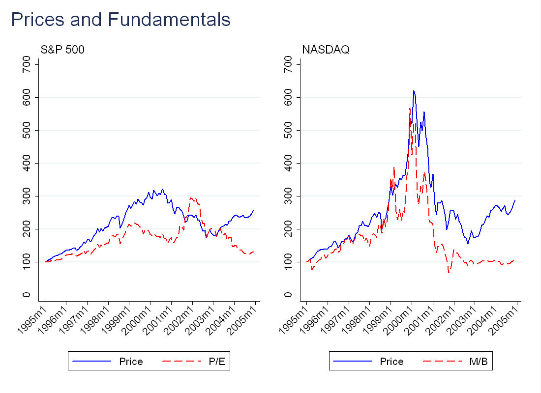
To understand if the Nasdaq was overvalued, I wanted to construct these measures for the Nasdaq 100, as well as the S\&P 500. An issue is that very few Nasdaq stocks paid dividends before 2003 (which makes sense - fast growing companies need to keep cash to reinvest in the business), so P/D will not be informative. Below, I describe exactly how I calculated P/E and M/B for the Nasdaq 100:
First, I used the Compustat index members database to find which firms were in the NASDAQ 100 on any given day. I then got data on book value of equity (I did not add investment tax credit nor subtract book value of preferred stock), dividends and EPS from Compustat and merged that with the index members. I used CRSP/Compustat merged to match this data with CRSP to get prices and returns. To compute the P/E and M/B for the index as a whole, I took the value-weighted average across all stocks in the index. For the plot below, I decided to go with M/B, as P/E is much noisier, so it’s harder to see exactly what’s going on (this makes sense, as earnings move more than book value of equity).
As for the S\&P 500, you can get EPS and dividend data directly from Compustat.
For all 4 series, I normalized the value in the first month (January 1995) to 100. Between 1998 and 2000, there is a big spike in the price and M/B ratio for the NASDAQ index, which collapses around 2001. This is not enough to say there was a bubble, just evidence that the stocks were expensive relative to fundamentals.

As an aside - there is a much more straightforward way to this for the whole Nasdaq, you can just download the CRSP data directly, and filter by exchange. I mention this because the paper uses the Nasdaq as a whole, not just the Nasdaq 100.

The Paper

The Question

There is no doubt that technology stocks went up a lot in the late 1990s and later fell. Although many people believe this was a bubble, the authors are not as convinced. Their goal is to develop an asset pricing model that can justify the rise and subsequent fall of Nasdaq stocks with rational expectations.

The Model

Although this is not the exact model used by the authors in the paper, it makes the same point in a simple fashion.
Consider a simple Gordon growth model: \begin{equation} \frac{P_t}{D_t}=E_t\left[\frac{1}{r-g} \right] \end{equation} where \(P\) is price, \(D\) is dividends, \(r\) is the discount rate and \(g\) is the average dividend growth rate. Note that \(\frac{1}{r-g}\) is convex in \(g\) (take a second derivative, and note the \(P/D\) is only well defined for \(r>g\)). This implies that increased uncertainty about \(g\) will increase the valuation (as measured by \(P/D\))
Consider two stocks A and B. A has a 1/2 chance of \(g=0\) and a 1/2 chance of \(g=0.1\), while B will have \(g=0.5\) for sure. Note that both firms have the same \(E(g)\). Now fix \(r=0.2\). Firm A will have a \(P/D\) of 7.5, while B will have a \(P/D\) of 6.67, so increased volatility increased valuation as desired.
Modeling the impact of uncertainty is important for understanding the Nasdaq. In the late 1990s, innovation lead to two main types of uncertainty: (1) Which technologies would be successful (2) Which firms producing a specific technology would be successful. The second point is interesting in its own right and will become the topic of a future post. The authors model this by allowing competition to arrive at any time \(dt\) with probability \(p \cdot dt\). In the model, arrival of this competitor sets the present value of the Nasdaq’s excess future earnings to zero.
Additional uncertainty was introduced by an increased number of IPOs, as well as firms going public earlier in their life-cycle. In these cases, investors had a small history upon which to base expectations, and were more uncertain about firm prospects.
Also note that the effect of uncertainty is amplified by a small equity premium, \(r\). In other words, the convexity of \(P/D\) is decreasing in \(r\). If we take the previous example, and bring \(r\) down from \(0.2\) to \(0.15\), we get that A’s \(P/D\) is 13.3 while B’s \(P/D\) is 5. The intuition for this is that when the equity premium is low, we discount the future by less, so a larger fraction of the present value comes from dividends in the far future. More weight on the future makes the present value more sensitive to uncertainty about dividend growth.
This is important, because around 2000, the equity premium was at historic lows. Fama and French (2002) find the average equity premium for 1951-2000 is 2.6-4.3, but their estimates for the premium in the year 2000 are as low as 0.32 (all of this is in annualized percentage terms).
The last piece of the story is explaining how well the model fits the data, which is discussed below.

Empirics

The authors ran into the same problem that I did with P/D - most of the stocks in their sample don’t pay dividends, so they focus on M/B ratio. Their model has a similar prediction to the Gordon growth model, however, in that M/B increases with uncertainty about the average growth rate of the firm’s book equity (also called book value).
In the first empirical exercise, the authors treat the Nasdaq as one large firm. They compute market value of equity and book value of equity by adding up across all the firms traded on the exchange, and divide one by the other to get M/B.
For a given level of expected excess return, the authors invert their pricing formula to find the book value growth rate uncertainty required to justify the observed M/B. They then find the corresponding return uncertainty associated with growth uncertainty , and compare this to the actual (realized) volatility.
Their main finding is that with an expected premium of 3% annually for Nasdaq stocks, the required model return volatility is 46.66% per year, very close to observed volatility of 41.49-47.03% (depending on calculation method).
The second part of the “bubble” is the burst, but their model can explain this as well. Nasdaq were not very profitable in 2000 and 2001. The authors explain that as uncertainty was resolved, agents revised their expectations for future growth downward, which caused prices to fall.
Actually, the model predicts an even larger decline than actually occurred in 2001, when the Nasdaq posted an average of -20% return on equity (ROE). This, however, was due to more than just poor operating performance, as many firms were taking large write-offs. Taking large write-offs signals that profits will be higher in the future, but they don’t model doesn’t account for this, so the authors believe the prediction is still valid.
The authors repeat this exercise with several individual firms, and find the same thing - the huge volatility required to justify a high price is often observed in the data. For example, using a -2% premium (the negative premium is needed to match the M/B) eBay would need a daily volatility of 129.24%, while the observed volatility was 113.64%.

Remarks

There are two points I want to make about the paper:
1) It’s important to note what the paper is actually doing. Under specific assumptions about how investors price assets, the authors can justify the high valuations in the Nasdaq under rational expectations. This is very impressive. But also very narrow. Given the increased media coverage, it’s reasonable to believe not all the people buying tech stocks were sophisticated investors (I am speculating here, and this should be the topic of a future post). I doubt all the investors (or rather, the marginal investor) really understood the uncertainty inherent in the Nasdaq stocks, nor did they behave as though the did.
2) Even if you don’t believe there was a bubble, there had to be something going on that was causing the extreme volatility (as mentioned above, the observed volatility was above 100%). As I continue to review more papers, hopefully this will become more clear.

Future Work

It is good to be skeptical about bubbles. As the authors mention, explaining something as a bubble is really not explaining it at all. That being said, there was something unique about what occurred in the 1990s in the Nasdaq (at least unique until you go back to the early part of the 20th century!). A combination of high valuations, high trading volume, and high volatility all suggest speculative behaviour. Just because rational expectations can explain what happened, doesn’t mean they do.