I recently recorded a series of video lectures for an introduction to Finance class at Kellogg. One of the topics we cover is the Capital Asset Pricing Model (CAPM). Recording this class got me thinking about the “beta anomaly” for the first time in years.

My initial interest in beta was near the end of the second year of my PhD program. I needed to write a second-year paper, and at the time, I was replicating the Betting Against Beta (BAB) paper by Frazzini and Pedersen. Although their paper is extremly well cited (at the time of writing, the BAB paper has over 1500 citations), I thought I could provide a different explanation for why low beta stocks tend to outperform high beta stocks. Although I never even self-published that paper, I think the results are interesting enough to post here on my blog.

In this post, I will provide a quick review of the CAPM, examine the returns of beta-sorted portfolios, and see how sensitive the results are to various sorting modifications. While I’ve personally constructed all these beta-sorted portfolios, rather than use my replication for the BAB factor in Frazzini and Pedersen’s paper, I will use the data published by AQR here.

Why Bet Against Beta?

There are two pieces of the CAPM. The first is the CAPM regression: \begin{equation} r_{i,t}-r_{f,t}=a_i + \beta_i (r_{m,t}-r_{f,t}) + e_{i,t} \end{equation} where \(r_{i,t}\) is the return on stock \(i\) at time \(t\), \(r_{m,t}\) is the return on the market, \(r_{f,t}\) is the risk-free rate and \(\beta_i\) is the CAPM beta. The CAPM regression tells us that moves in the market might be able to explain some of the moves in stocks, but there is error i.e. moves in stocks not explained by the market, \(e_{i,t}\). This error is firm-specific risk, and the CAPM puts no restriction on how large its variance, \(Var(e_{i,t})\), can be. The main use for the CAPM regression is to estimate \(\beta_i\) and use it in the CAPM equation: \begin{equation} E[r_i]=r_f+\beta_i MRP \end{equation} where \(MRP\) is the market risk premium i.e. the compenstion for bearing market risk. In a future post, I will talk about how we might measure the market risk premium. In the CAPM equation, there is no error: stocks with higher betas should have higher expected returns. And this is the only reason stocks should have different expected returns.

Empirically, however, the opposite is true: low beta stocks tend to have higher (risk-adjusted) returns than high beta stocks. There are many explanations for this failure of the CAPM, but one of the most well known is explained in Capital market equilibrium with restricted borrowing, by Fischer Black (1972). This paper argues that the beta anomaly exists because one can not actually borrow/lend unlimited amounts at the risk free rate (an assumption required for the CAPM to hold). To achieve high returns with low beta stocks, an investor whould have to apply leverage, which is not cheap (unless you are Warren Buffett). So, with limited leverage, investors can only achieve high returns with high beta stocks. This leads to excess demand for these high beta stocks, pushing up their prices, and pushing down their expected returns. Limits on leverage are also the key mechanism in the theoretical model in the BAB paper.

There are other explanations for the beta anomaly, e.g. that it is demand for lottery-like stocks (see e.g. Bali, Turan G., et al. “Betting against beta or demand for lottery.” (2014)) or that it is the result of non-standard sorting procedures (see e.g. Novy-Marx, Robert, and Mihail Velikov. “Betting against betting against beta.” (2018)). I am more sympathetic to the non-standard sorting procedure argument, as there are a few things in the BAB paper that seemed unusual when I was first reading it: (1) Not using value weights (2) Applying time-varying leverage to the long and short sides of the portfolio.

In the next few sections, I will go through how I would form these portfolios, then I will examine the effects of changing the weights, and adding the time-varying leverage. Going through these non-standard sorting procedures will reveal something interesting about the BAB strategy.

Basic Sorting

I start by calculating each firm’s CAPM beta over the past year using daily returns (I require that a firm have at least 126 non-missing daily returns in this calculation to be included in my sample). I then follow Hou, Xue and Zhang (2020), and form 10 value-weighted portfolios based on NYSE breakpoints. In this, and all future analysis, I restrict to ordinary common shares traded on major exchanges. Finally, I form a long short portfolio by subtracting the return of the high beta portfolio from the return of the low beta portfolio.

I am going to evalue these portfolios three ways (1) the mean (2) the Sharpe ratio, which is the mean, minus the risk-free rate, devided by the standard deviation i.e. how much additional mean return you are getting for each unit of risk and (3) the 3-Factor alpha, which is the constant in a regression of the portfolio returns on the market, size and value factors i.e. how much mean return is not explained by these three factors.

Here are the annualized mean, Sharpe ratio and 3-Factor (market, size and value) alpha for the 10 beta-sorted portfolios: 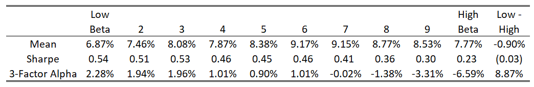In the first row, the CAPM doesn’t look like a total failure… high beta stocks do have higher returns, but it tends to peak around the 6th and 7th portfolio. The real difference is in the risk-adjusted returns. The 3-Factor alpha of the long short portfolio is almost 9% a year, which is huge!

Weights

In the BAB paper, they use beta weights, rather than value weights. I talked about the issues with using beta weights in a previous blog post. Still, I was curious what would happen if we use equal-weighted portfolios instead of value-weighted portfolios. Here are the results with 10 equal-weighted portfolios: 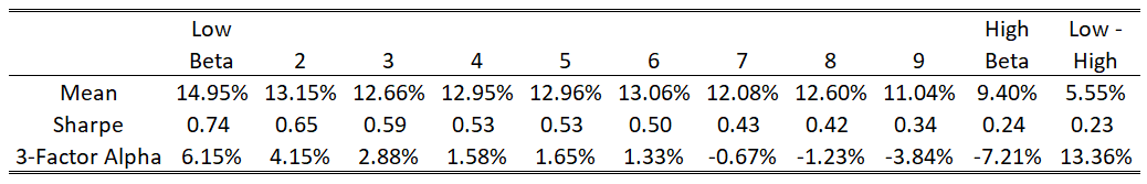Now the beta anomaly appears even stronger. The low beta portfolio actually has higher mean returns than the high beta portfolio, a total failure for the CAPM. We’ve also increased the alpha to over 13% per year.

Making the Portfolio Market Neutral

As I’ve constructed it so far, the long short portfolio is not necessarily market-neutral i.e. the expected beta of that portfolio may not be zero. Frazzini and Pedersen propose a procedure to remove all (expected) market risk from the BAB portfolio.

First, shrink all betas toward one \(\beta_{new}=0.6 \times \beta_{past year}+0.4 \times 1\) (with the idea that the mean cross-sectional beta must be one). Then, compute the value-weighted average \(\beta_{new}\) for each portfolio. Finally, take the return of the each portfolio portfolios, and multiply it by one over the (value-weighted) average beta. This will increase the leverage on the low-beta portfolio, and decrease leverage on the high beta portfolios. If betas were constant, every portfolio would have a beta of one. I will call multipling portfolios by \(1/E[\beta_{new}]\) the beta one adjustment. This also means that the long-short portfolio should have an expected beta of zero.

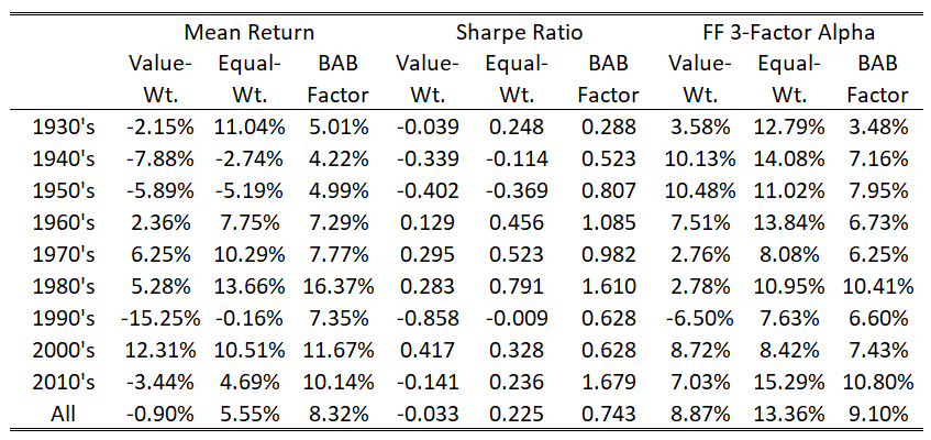
Here are the results for the 10 value-weighted portfolios, but setting the expected beta of each portfolio to one: 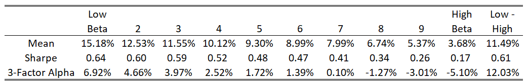Now the beta anomaly is even stronger. The low beta portfolio has a return over 11% higher per year than the high beta portfolio.

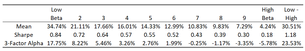
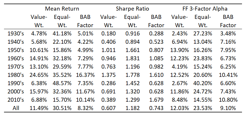
The effect gets downright huge when we do this with the equal-weighted portfolios:

Time-Varying Leverage

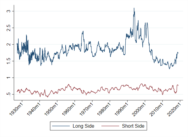
Making the long-short portfolio market neutral is putting time-varying weights on the long/short sides of the portfolio. The tables above show that this time varying leverage matters a lot for the size of the beta anomaly. While this is too much to get into for a blog post, I believe it has to do with the fact that betas compress toward one in bad times, so this would trim leverage when we would expect the market as a whole to perform poorly.

This table shows the average weight on the long/short side by decade:

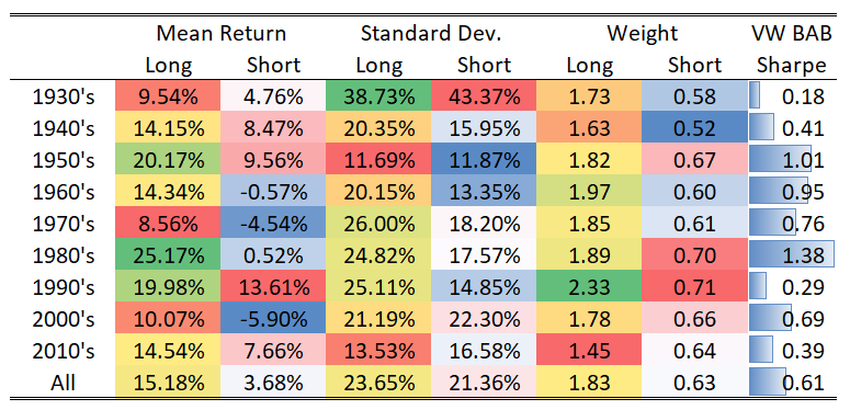
And here is a plot with the leverage by month:

Time Period

Looking at the leverage over time made me want to understand if the beta-sorted portfolios do particurlarly well in and decade. Here are the mean returns, Sharpe ratios and alphas of the long-short portfolios I’ve constructed:

Nothing really stands out to me here, but what happens if we apply the beta one adjustment?

Now we have the value-weighted factor having positive mean return, Sharpe ratio, and alpha in every decade. So betting against beta seems to have been consistently profitable. But, for this to be true, we need to make the beta one adjustment.

Embedded Options

The explanation I put forth in the paper was that the the time-varying leverage makes the portfolio look like an option-writing strategy. Here is a plot of the monthly returns each long-short portfolio against the market: 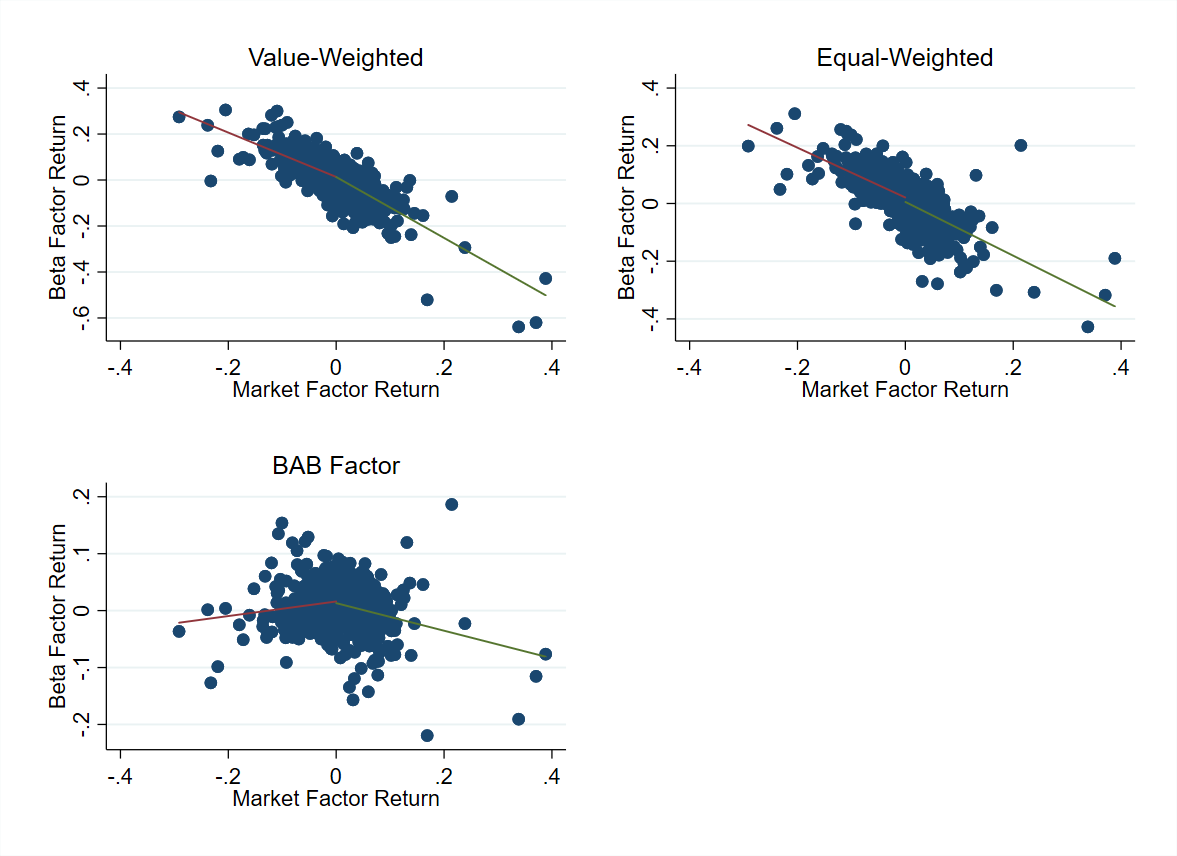Note that the BAB factor actually looks somewhat like a bet against volatility. It has higher returns when the market has a return close to zero, and lower returns otherwise. This is not true, however, for the value-weigthed or equal-weighted strategies I constructed.

Here is the same picture, applying the beta one adjustment to my portfolios: 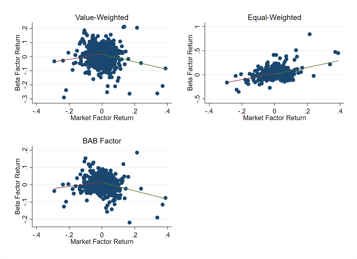We can see that this is the secret sauce which makes the long short portfolio look like a short straddle.

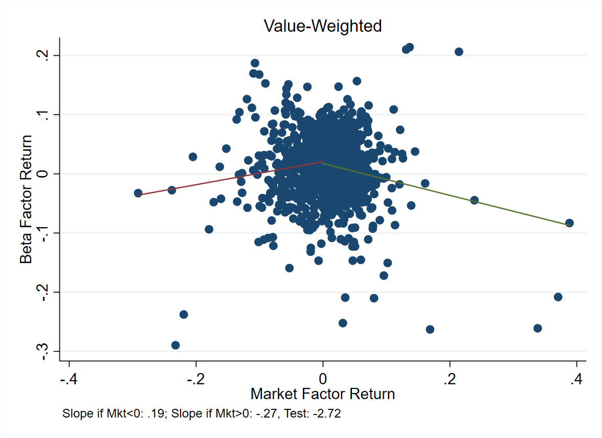
The slope are statistically significantly different depending on whether the market has a positive or negative return:

Now, why is this happening? 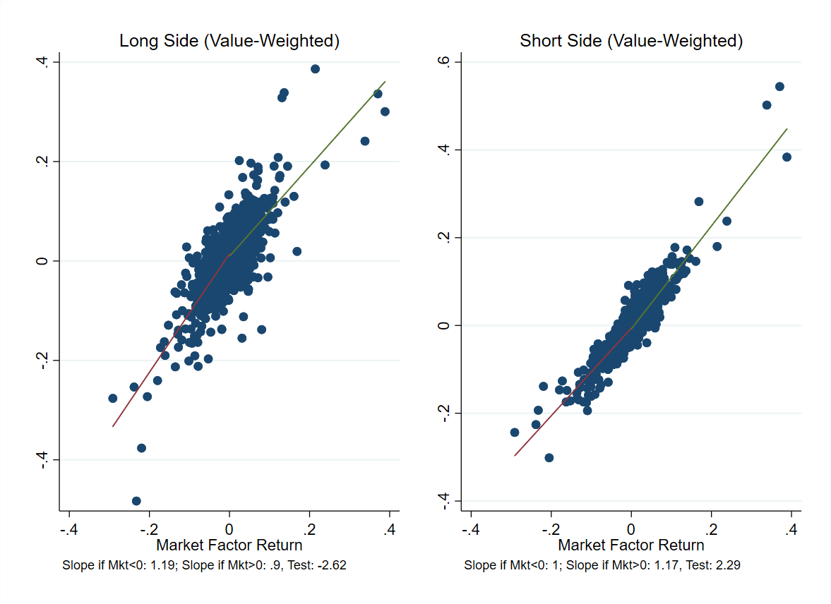The long side looks like the market plus a short call. The short side looks like the market plus a long call. So it seems like there are embedded options in these strategies. Now, why would this earn a premium? It is well documented that option-writing strategies earn a premium see e.g. Jurek and Stafford. “The cost of capital for alternative investments.” (2015). My propsed explanation that the alpha in BAB was due to an embedded option-writing strategy embedded in the portfolio.

Wrap Up

I think the evidence here makes it clear that there is something special about the BAB portfolio constructed by Frazzini and Pedersen. The basic value-weighted long-short beta portfolio has a negative mean. But, when we use equal weghts, or apply the time-varying leverage to the long and short sides, we can get a large positive mean. We also get an interesting pattern: the BAB portfolio, constructed using only equities, has payoffs that look like an option-writing strategy. I think this is why people are still studying the beta anomaly over 40 years after Fischer Black’s paper – it is not clear whether or not it really exists, and if it does exist, why it occurs!